D-c FLUX

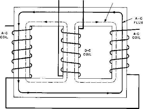Fig. 205. Windings and core flux paths in a saturable reactor.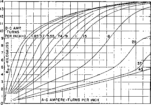

2 4 6 8 10 12 14 16 18 20 ZZ 24 26 28 30 32 34 36 36 40

Fig. 206. Magnetization curves for 4% silicon steel.

ductance is halved and the alternating current doubled, core leg shunts the even harmonics of a-c fiux.

Rectangular B-H loops are obtained in grain-oriented core materials. It is only in these materials that the wave shapes of Fig. 204(a) are even approximated. In unoriented core steel, wave shape is much more rounded, and control current bears less resemblance to load current. Figures 206 and 207 indicate the contrast in saturation control afforded by unoriented silicon steel and oriented nickel steel. In

О

О

о о

Nl/lN BASED ON TURNS AND I (AMPS) FOR ONE TOROID

0 10 20 30 40 50

LOAD A-C NI/IN

Fig. 207. Typical magnetization curves for 0.002-in. grain-oriented nickel-steel

toroidal cores.

grain-oriented steel cores there is an approximately linear relationship between d-c ampere-turns per inch and a-c ampere-turns per inch over a large range of flux density. Moreover, the a-c iV in. for a given d-c iV in. change but little with a-c flux density over this range. In Fig. 207, each of the lines for a given value of control magnetizing force is nearly vertical. For a given value of control iV in., load current is almost independent of flux density and therefore of a-c supply voltage. The sections following are based on the use of grain-oriented core steel.

111. Graphical Performance of Simple Magnetic Amplifiers. Since with a given core and supply frequency there corresponds a definite voltage for every flux density, and since for a given number of turns the ampere-turns per inch are proportional to current, the curves of Fig. 207 may be replotted in terms of voltage and current. We may then plot load lines on these curves in a manner similar to those in electronic

The middle

amplifiers, so that the operation, efficiency, control power, etc., may all be determined from a study of these load lines.

In Chapter 5 (p. 142) equation 58 indicates that the a-c voltage in a vacuum-tube circuit is divided between the load and the tube. If a resistive load is used, a straight line can be drawn on the characteristics of a vacuum tube which will form the locus of plate current and plate voltage for any given load and supply voltage. This line is called the load line, and by use of it the gain and power output of the amplifier can be determined.

A-c MAGNETIZING FORCE AMPERE TURNS PER INCH

ш

v> I- i о >

< z о:

1.6 1.4 1.2 1.0 .8 .6 .4 .2

<

о о

14 =!

12 к

Ю t v>

о

N1=AMPERE TURNS

YiQ. 208. Geneiahzed magnetic amplifier characteristics and load Ime.

A similar method can be used with magnetic amplifiers. If a linear reactor were connected in series with the load, the voltage across the load and the voltage across the reactor would add at right angles. With rectangular loop core materials, currents are not reactive in the linear sense, so that the actual load line is neither a straight line nor an ellipse. For practical calculations the straight line is used, and the results obtained are correct within small percentages if the reactor \ oltage and current are measured on an average-reading voltmeter and ammeter.

Figure 208 shows similar information to Fig. 207, except that it is for a given core. The scale of abscissas is ampere-turns, and the scale of ordinates is volts per turn. These characteristics can be used for any amplifier which uses the same cores and the same supply voltage and frequency as the amplifier on which the measurements

were made to obtain these characteristics. These characteristics can be derived for a given core from the parameters of a-c flux density, a-c magnetizing force, and d-c magnetizing force as shown to the right and top of Fig. 208. These curves then give a set of characteristics for a given core rather than for a given core material. Some error is involved if these curves are used with a different supply frequency from the one used in making the original curves. Over a narrow range of frequency the curves of Fig. 208 using the scale at the top and to the right can be used to determine the operation of a magnetic amplifier for different loads. The curves of Fig. 207 may be used for magnetic amplifier calculations in this manner. For convenience of calculation, it is usually preferable to make a set of characteristic curves for several core sizes and for each supply frequency.

An example will show how these curves can be used in the design of magnetic amplifiers. Assume that it is necessary to design an amplifier with 30 watts output using cores with E/N and NI of Fig. 208. The supply voltage is 100 volts, the load is 200 ohms, and 0.01 amp is available for use in the control winding. The characteristics show the E/N can be varied from about 1.4 to 0.2 and still stay on the linear part of the characteristic curves. The power output is equal to /E X I which is also equal to A {E/N) X AAV, where E is the alternating voltage across the reactors, / is the alternating current through the reactors, and N is the number of turns in the load windings of the reactor. AiY/ needed for 30 watts = 30/(1.4 - 0.2) = 25 ampere-turns. Load impedance is AE/AI. A load line on Fig. 208 is (AE/Nl) aNI = (aE/aI) (1/AV), where Nl = turns in load winding. For 200 ohms, the load line passes through the points E/Nl = 1.4, NIc ~ 2.5, and through E/Nl = 0.2, NIac = 27.5. When this line is extended to the ordinate it intersects at 1.54. This is the point of zero alternating current or of infinite reactor inductance. At this point the total supply \ltage would be across the reactor. Since the supply voltage is 100 volts, 100/A = 1.54 and Nl = 65 turns. By interpolation of the d-c NI curves, we see that, for E/N = 0.2 and Nhc = 27.5, 25 ampere-turns are necessary in the control winding. The turns in the control windings are NJc/h = 25/0.01 = 2,500 turns. Here Ic is the current in the control winding, and Nc are the turns in the control winding. Control winding resistance is determined by the wire size. For the purpose of this example, assume that the resistance of the control winding is 500 ohms. Then the power in the control winding is 500 X = 0.05 watt. Power gain of the amplifier is power out/ power in = 30/0.05 = 600. The impedance of either the input cir-

cuit or output circuit can be changed by changing the number of turns in the respective windings. Either impedance varies with the square of the number of turns used in the winding. For example, the load line which was used for 200 ohms in the preceding example could be used

for 800 ohms. The load winding would then have V §00/200 X 65 = 130 turns, and the supply voltage would be 200 volts instead of 100 for E/N = 1.54 at zero current.

Power output is proportional to the area of the rectangle of which the load line forms a diagonal. More power output can be obtained by using a load line with less slope, but gain may increase or decrease, depending upon the winding resistances and core material. In the

LINE VOLTAGE 120 110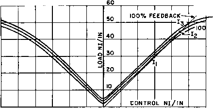

-60 -50 -40 -30 -го -10 0 10 20 50 40 50 60

Fig. 209. Simple magnetic amplifier transfer curves with line-voltage variations.

preceding example, the load windings were assumed to be in series with the load, as in Fig. 203. This is the connection commonly used when the source is a 60-cycle a-c line. With a high impedance source, it is preferable to connect the load \vindings in shunt with the load. Then the ordinates of Figs. 207 and 208 correspond to load voltage at all times.

If we choose three line voltages corresponding to flux densities within the linear portions of Fig. 207, and plot the d-c control versus a-c load ampere-turns per inch, the curves of Fig. 209 result. If, instead of Nl/in., a\erage load current is plotted, Fig. 209 gives the transfer curves for a simple magnetic amplifier. The curves are symmetrical about zero ampere-turns. The difference between the transfer curve and a straight line indicates the degree of non-linearity in the amplifier for any load current. With grain-oriented core material the a-c load current is nearly independent of supply voltage for a-c inductions less than saturation. Provided that appropriate changes

in scale are made, transfer curves may be plotted between load voltage and control current, or between load ampere-turns and control ampere-turns, or between combinations of these.

Load current is the result of flux excursions beyond the knee of the normal magnetization curve. In Fig. 207 the curve for zero control Nl/m. is normal magnetization for the material. When direct current flows in the control windings, it sets up a constant magnetizing force in the core. Then superposed a-c magnetizing force readily causes a flux excursion beyond the knee of the curve, permeability suddenly drops, and a large current flows through the load winding. The point in the voltage cycle at which this sudden increase in current occurs depends upon the amount of direct current in the control winding. Magnetic amplifiers with steep current curves like those of Fig. 207 can be used as control relays.

Load current is usually measured with an average-reading ammeter, such as a rectifier-type instrument. This kind of ammeter is generally marked to read the rms value of sinusoidal current but actually measures the average value. Thus the ammeter reading is 0.707/0.636 = 1.11 times the average current over a half-cycle. When the meter is used to measure non-sinusoidal current, it still reads 1.11 times the average.

Except for the slight amount of non-linearity noted in Fig. 209, the average value of ampere-turns in the load winding of each reactor equals the d-c ampere-turns in the control winding. But since the a-c ammeter reads 1.11 times this value, the load a-c iV7/in. are 1.11 times the control d-c iV in., plus the differential due to core magnetizing current. Thus, if a core had infinite permeability up to the knee of the magnetization curve and zero permeability beyond the knee, the transfer curve would be exactly linear. Oriented nickel-iron alloy cores approach this ideal and therefore are more nearly linear than other materials.

112. Response Time. Because of the inductance of the reactor coils, when a change is made in the control winding direct current, load current does not change immediately to its final value. An interval of time, called response time, elapses between the change in control current and the establishment of a new steady value of load current. If the inductance were constant during the change, the response time constant would be the time required for a load current increase to rise to 63 per cent of the final value after a sudden control current increase. Magnetic amplifier response time cannot be evaluated as an

(112)

Rc 4fRc \Nb/

where Та = time for load current increment to reach 63 per cent of final value

Lc = equivalent total control coil inductance (henrys) Rc = total control circuit resistance (ohms) Rl = load resistance / = line frequency Nc = turns in control Avinding Ni = turns in load winding.

An obvious method of decreasing magnetic amplifier response time is by increasing Rc, but this has the disadvantage of reducing overall power gain. Gain and response time are so related that the ratio of gain to time constant in a magnetic amplifier is usually given as a figure of merit.

113. Feedback in Magnetic Amplifiers. If a rectifier is interposed between the reactor and load, and a separate winding on the reactor is connected to this rectifier as in Fig. 210, it is possible to obtain

load wdg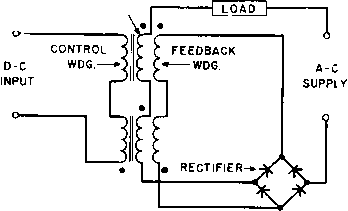

Fig. 210. Magnetic amplifier with external feedback.

sufficient power from the rectifier to supply most of the control power. If the control power from the rectifier furnishes the ampere-turns represented by the straight line in Fig. 209, the amplifier is said to

1 Transient Response of Saturable Reactors with Resistive Load, by H. F. Storm, Trans. AIEE, 70, Part I, p. 99 (1951).

ordinary linear L/R time constant. Storm shows that the time of response of simple magnetic amplifiers is independent of core permeability. An average or equivalent control circuit inductance may be found from the relation

Lc Rl /NcV

have 100 per cent feedback. It is then necessary for the control winding to supply only the amount represented by the horizontal difference between the transfer curve and the straight line. This greatly increases the amplification of a pair of reactors.

Typical transfer curves for a simple magnetic amplifier are plotted in Fig. 209 for three a-c supply voltages: 100, 110, and 120 volts. A 100 per cent feedback line intersects the transfer curves at Ii, I2, and /3, respectively. The control Nl/in. are furnished by the feedback, except for the control current difference between the feedback line and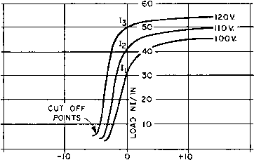

CONTROL Nl/lN

Fig. 2П. Transfer curves for magnetic amplifier with feedback.

the transfer curve. Positive control current is required when the transfer curve is at the right, and negative current when it is at the left, of the feedback line. Net control iY7/in. for the three voltages are plotted in Fig. 211 with expanded abscissa scale. Now the transfer curve is asymmetiical. Most of the amplifier gain occurs with negative control current changes. On the steep parts of the transfer curves, gain is fairly linear and greatly exceeds the gain of simple amplifiers. Below the steep parts, output current reaches a minimum but remains small with relatively large excursions of negative control current. These current minima are called cut-off points. Reference to Fig. 207 shows that cut-off current is /дт, the normal exciting current at supply voltage E. With positive control, current output levels off to a nearly constant value, depending on the voltage. Feedback causes output current to be quite dependent on variations in a-c supply voltage, because has a greater effect than in simple amplifiers.

Computing control current for transfer curves with feedback as described in the preceding paragraph involves a small difference between two large quantities. Minor measurement errors in the original

data cause large inaccuracies in the feedback transfer curves of Fig. 211. A more accurate derivation of 100 per cent feedback transfer curves is given in Section 117.

To the left of the cut-off points, the transfer curve rises slowly toward the left along a straight line, as in Fig. 212(a). This line corresponds to 100 per cent negative feedback; it is practically linear, but gain is much reduced. The transfer curves of Fig. 211 would, if continued to the left, merge into such a line.

Polarities in Fig. 210 are for positive feedback with positive direct current entering the control winding at the top. Negative feedback is obtained if the control current is reversed. If series feedback is derived as shown in Fig. 210, the feedback current is Еь/Rl- It is possible to connect the feedback circuit across the load to obtain voltage feedback. To conserve power, the feedback resistance should be large relative to R.

114. Bistable Amplifiers. Positive feedback in a magnetic amplifier can be increased to more than 100 per cent by increasing turns in the feedback winding. Transfer curves may then become double-valued and give rise to abrupt load current changes with changing control current. Such amplifiers are called bistable. In Fig. 209, the effect of increasing feedback would be to decrease the slope of the feedback line. If the feedback were increased gradually, operation would remain stable until the feedback line had the same slope as the transfer curve. Then the load current would become some indefinite value along the transfer curve. If the feedback were increased further stable operation луоиЫ be had at only one of two values of load current. Bistability is illustrated in Fig. 212(a). Here a transfer curve similar to those of Fig. 211 is shown except that it is with load voltage ordinates and expanded Ncc abscissas. The amount of feedback in excess of 100 per cent is drawn as line AB with slope less than that of the main part of the 100 per cent feedback transfer curve. Another line, CD, is drawn parallel to the line AB. These lines are tangent to the transfer curve at points A and C- With feedback > 100 per cent, let d-c control current be decreased from some negative value toward zero. Load voltage or current follows the transfer curve until it reaches point A; then it jumps to point B, and further increase of control current results in very little load voltage increase beyond point B. If control current is subsequently reduced, load voltage follows the top of the transfer curve until it reaches point C; then it drops abruptly to point D.

Bistable action is shown in Fig. 212(6) as a function of control Nl/m with points A, B, C, and D corresponding to those in Fig. 212(a). Line AB in Fig. 212(a) represents feedback ampere-turns Nflf in excess of 100 per cent, which are proportional to E. Line AB extended intersects the axis of abscissas at F% and CD extended intersects at G. Vertical lines erected at A and F intersect the transfer

TRANSFER CURVE FOR 100% FEEDBACK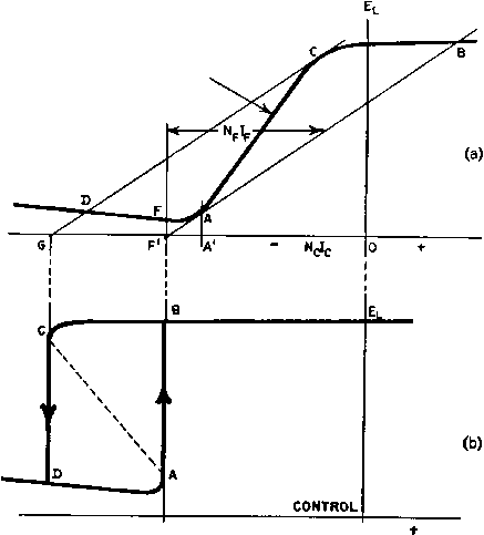

Ncic 0

Fig. 212. (a) Typical transfer curve, and (b) bistable magnetic amplifier.

curve at A and F, respectively. FA represents ampere-turns Nflf when control ampere-turns NcIc are at point F. When decreasing negative NcIc reach value F, the load voltage jumps from A to B, Points F and G are projected downward to Fig. 212(6). In this figure the output jumps to final value B, but the increase actually takes place along the dotted line. Decreasing additional feedback Nflf reduces the differential amount FG of control NcIc and reduces the width of the bistable loop. Coniersely, increasing Aflf widens the loop and provides a greater margin for variations in Nflf due to voltage, temperature, etc. Bistable amplifiers are used in protecti\x and control circuits to turn relays or indicators on or off wben control