power varies between narrow limits and the inherent loek-in action is desirable.

115, Current Transductors. In some countries the term transductor is used to denote any magnetic amplifier. Here it denotes a saturable reactor circuit for measuring direct current. A current transductor is hardly an amplifier; it is a metering device. A transductor circuit is shown in Fig. 213. It is similar to that of Fig. 210 but with feed-

LOAD

TO D-C SUPPLY

A-C SUPPLY

Fig. 213. Current transductor circuit.

back windings and a-c load removed. Operation is entirely different. Cores are circular or square, and are wound in-and-out toroid-ally in a manner resembling through-type current transformers. The heavy d-c bus then may be inserted through the toroid to form a single turn on each core. In Fig. 213 the d-c load windings are shown aiding, and the a-c windings bucking; this accomplishes the same core flux polarities as for Fig. 205. Load direct current is determined by the load resistance, which is large compared to the reactance of the transductor. Control circuit impedance multiplied by the turns ratio is large; magnetization is constrained. It will be recalled from Section 110 that, under this condition, even current harmonics cannot flow. Therefore a-c winding current is flat-topped. After this flat-topped current is rectified, it flows through the ammeter as smooth direct current.

At any instant one reactor of the pair is saturated, and the other unsaturated. On each a-c half-cycle the unsaturated reactor maintains the output current constant. Total output d-c ampere-turns of course must equal twice the load direct current at all times. Transductors are like simple magnetic amplifiers as far as the relations of load and output currents are concerned. They have been built to measure currents of 10,000 amp or more, with good linearity.

J For a description of the current and flux conditions, see Mngnoic Amplifiers, by S. E. Tweedy, Electronic Eng., February, 1948, p. 38.

control input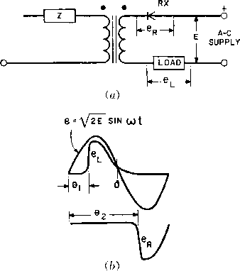

Fig, 214. (a) Half-wave self-saturated magnetic amplifier circuit and (b) load

and rectifier voltage wave shapes.

be formed. Impedance Z in the control circuit prevents short-circuiting the reactor. It may be the control winding of another reactor in a practical amplifier. Rectifier UX prevents current flow into the load in one direction, so that the core tends to remain in a continually saturated condition. This condition is modified by negatiл^c control winding AV/in., which opposes the load winding .¥ in. and permits the core to become unsaturated during the portion of the cycle when there is no load current flowing. The greater the control AV/in., the less the average output current. Transfer characteristics are similar to those of Fig. 211. Ideally the circuit has 100 per cent feedback.

Assuming the core to be saturated at all times with zero control current, current flows into the load throughout the whole positive half-cycle and is zero for the whole negative half-CTcle. With a given

116. Self-Saturated Magnetic Amplifiers. In Section 113 it was seen that the use of feedback windings greatly increases the gain of a magnetic amplifier. Several circuits have been devised to provide the feedback by means of the load circuit and thus eliminate the extra feedback winding. Such circuits are termed self-saturating. A building-block or elementary self-saturating component is the half-wave circuit of Fig. 214, from which several magnetic amplifiers may

value of negative control current, reactor inductance is high at the start of the positive half-cycle and load current does not build up appreciably until an angle Oi is reached when the core saturates. Then it climbs rapidly and causes most of the supply voltage to appear across the load as shown by the curve marked in Fig. 214(b) for the remainder of the positive half-cycle. As negative control current increases, so does angle <9i. In the limit Oi = 180°; that is, with large negative control current, virtually no load current flows. The similarity of load voltage wave shape to thyratron action is at once evident. It has led to the use of the same terminology. Angle Oi is often called the firing angle of a magnetic amplifier. Load voltage is reduced as (9i increases, approximately as in Fig. 190. There are some important differences, too:

(a) Reactor inductance is never infinite, and magnetizing current is therefore not zero. This means that during the interval O-i a small current flows into the load. The change in reactor inductance at the firing instant is not instantaneous; the time required for the inductance to change limits the sharpness of load current rise.

(b) Even with tight coupling between control and load windings, the saturated reactor inductance is measurable. This saturated inductance causes the load current to rise with finite slope.

(c) After load voltage reaches its peak and starts to drop along yviih the alternating supply voltage e, core flux continues at saturation density. An instant a is reached when the load voltage exceeds the supply voltage. Beyond a, the reactor inductance increases and magnetizing current decreases, but at a rate slower than the supply voltage because of eddy currents in the core.

(d) After supply voltage e in Fig. 214(b) reaches zero, the reactor continues to absorb the voltage until the core flux is reset to a \alue dependent on the control current, that is, until angle 82 is reached. Then part of the negative supply voltage rises suddenly across rectifier RX as shown by the wave form of e.

During the interval O-i the reactor inductance is high and virtually all the supply voltage appears across it. The voltage time integral

je dt represented by the reactor flux increase during this interval is

equal to Jedt during 7г-2- That is, the energy stored in the core

before the firing instant is given up during the negative half-cycle of supply voltage.

Self-saturated magnetic amplifiers have transfer curves similar to that of Fig. 212(a). A small amount of additional positive feedback makes them bistable. Negative feedback makes the transfer curve more linear but reduces the gain. Ordinates and abscissas may be current, ampere-turns, or oersteds, as for simple magnetic amplifiers.

117. Hysteresis Loops and Transfer Curves. Several workers have observed that the transfer curves of Fig. 211 are similar in shape to the left-hand or return trace of the hysteresis loop. There is a con-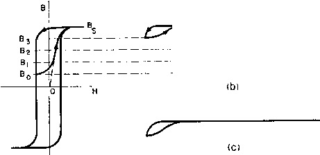

Fig. 215. Minor loops in rectangular hysteresis loop core material.

nection between the two. In Fig. 21, p. 25, it was shown that in a core with both a-c and d-c magnetization the minor hysteresis loop follows the back trace of the major loop in the negative or decreasing В direction, and proceeds along a line with less slope in the positive direction until it joins the normal permeability curve at B- Also, it was pointed out in connection with Fig. 69, p. 94, that, if AB has the maximum value B, , the result is the banana-shaped figure OBD. Here again the loop representing flux excursion О-В^, follows the left-hand side of the hysteresis loop in the downward or negative direction. In a rectangular hysteresis loop material with B-H loop shown in Fig. 215(a), the path traced over a flux excursion BBg is more irregular in shape but still follows the left-hand trace of the loop. If magnetic amphfier cores are biased to a series of reset flux positions Bq to Bi the corresponding flux excursions and minor loops are those shown in Fig. 215(b). Usually, the load current far exceeds the control current necessary to reset the cores, so that these loops actually have a much longer region over which the loop width is practically

1 See Self-Saturation in Magnetic Amplifiers, by W. J. Doi-nhoefer, Tram. AIEE, 68, 835 (1949).

Under the assumptions, equation 1 becomes

r- N ёф

V2 Esmwt = for 0 < ict < co/i (11-1)

10 dt

zero, as shown in Fig. 215(c). This is true of all the loops regardless of flux excursion.

The foregoing is true of a slowly varying flux excursion, so that the locus of the lower end points of the minor loops is the left-hand trace of the d-c hysteresis loop. Most magnetic materials, including rectangular loop materials, have a wider loop when the hysteresis loop is taken under a-c conditions, because of eddy currents. The difference between loops is as shown in Fig. 216. The locus of the end points of the minor loops under a-c flux excursions is neither the a-c nor the d-c loop but an intermediate line such as that drawn dot-dash in Fig. 216. The slope of this line is less than that of either the a-c or the d-c loop, and the gain of the magnetic amphfier is accordingly reduced.

An analysis for the self-saturated magnetic amplifier of Fig. 214(a) is given below. Load current is assumed to have the same shape as вь in Fig. 214(b), and the following assumptions are made:

1. Sinusoidal supply voltage and negligible a-c source impedance.

2. Negligible reactor and rectifier forward voltage iR drops.

3. Negligible rectifier back leakage current.

4. Negligible magnetizing current compared to load current.

5. Negligible saturated inductance.

6. High control circuit impedance.

1. E = 4..ЩХфе X 10 (113)

This will be recognized as equation 4 (p. 6) with peak flux at saturation value Other terms are listed as follows:

(Л

о о

=! -4 -8 -12 -16

d-c loop

A-c lo6p-*4

locus of

-1.0

h-oersteds

Fig. 216. D-c and a-c B-H loop.s for grain-oriented nickel steel.

Integrating equation 114 gives

10-* Г V = Г V2

E sin rfi

= 1 - COS 0)t]

(115)

(116)

(117)

(118)

V2E X 10* During the interval < < w, load voltage is

V2 E sin = zi?L where is the load resistance. This may be integrated to give

J -1(11 I + cos coti

Combining equations 116 and 118 and substituting equation 113,

idt= -iфs Л-Фо)Х 10- (119)

The left side of equation 119 is the average load current over the conducting interval тг/со - ti. Average load current over the whole cycle is

Equation 120 has two flux terms: фs, which is a fixed quantity for a given core material; and фо- The relation between фо and control

12 8 4

current is, as indicated in Fig. 215, the return trace of the major hysteresis loop. Thus equation 120 states that the average load current is the sum of a constant term and a term which has the same shape as the return trace of the hysteresis loop. Quantitatively, a self-saturated half-wa\e magnetic amplifier has a current transfer curve the same as the return trace of the core hysteresis loop, except that ordinates are multiplied by JAcN/IORl and are displaced vertically by an amount jBAcN/WRl-

Comparison with equation 113 reveals that the ordinate multiplier and vertical displacement are E/4:A4:RlBs and E/4:A4:Rl, respectively. As noted above, the return trace should be modified to mean the dot-dash line of Fig. 216.

118. Self-Saturated Magnetic Amplifier Circuits. In Fig. 217 three single-phase circuits are diagrammed which comprise two of the half-

D-C INPUT

о

С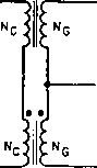

(d) DOUBLER CIRCUIT

D-C INPUT

(b) BRIDGE CIRCUIT

D-C INPUT

О E o-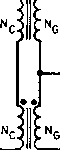

o E o-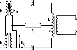

(C) CENTER-TAP D-C OUTPUT CIRCUIT

Fig. 217. Self-saturated magnetic amplifier circuits,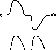

the control chcuit and influence the °

wave elements described in the preceding sections. These circuits are discussed briefly below.

(a) Doubler Circuit. This is really two half-wave circuits working into a common load. Rectifier polarities are such as to cause a-c voltage to appear across the load, as in Fig. 218(a). The wave shape departs somewhat from alternately reversed half-waves. In the doubler, the reactor which is carrying load current during a given half-cycle causes a reduction in the resetting voltage, and therefore in the time rate of resetting flux change of the other reactor. This increases the output and gain for a given control current compared to the half-wa\e circuit but has no effect on current minima at the cutoff points (see Fig. 211).

When control circuit resistance Rc is large, the control current and associated magnetizing force are fixed, but, when Rc is small, even harmonic currents flow freely in

wave shape for a given control current F. 218. Single-phase mag-j n 1 1 i- J. netic amplifier output; (a)

further. Generally, low values of resist- , , .

. . , a-c voltage across load; [b)

ance Rc cause a slight increase m the con- yoitage across load,

trol oersteds for a given output but virtually no change in slope. In other words, the whole transfer curve is displaced slightly to the right.

(b) Single-Phase Bridge Circuit. Here two extra rectifiers isolate the two reactors at all times, and the wave form is like that of the half-wave rectifier, except that it occurs twice each cycle. Load current is d-c; that is, both reactors produce load current of the same polarity, as in Fig. 218(b). Because of the isolation of the two reactors, the transfer curve closely follows a dot-dash line like that in Fig. 216 if the core is grain-oriented nickel steel, or a similar line between a-c and d-c loops for other core material. Control resistance Ra affects output in a manner similar to that mentioned for the doubler.

(c) Center-Tap D-C Circuit. Although the reactors are not isolated in this circuit, load and resetting currents are still the same as for the bridge circuit, and hence the transfer curve has the same shape, unless the rectifier reverse currents are appreciable. Then gain is appreciably reduced.

In all these single-phase circuits, the load current is twice that of

the half-wave cnxiiit. Therefore transfer curves may be predicted from B-H loops as in Section 117, but ordinates are multiplied by E/222RlBs, and the \ertical displacement is E/2.22Rl. From these multipliers it can be seen that output current is proportional to supply voltage E, and tlicrefore power gain is proportional to E. In this respect, a self-saturated amplifier contrasts with a simple magnetic amplifier, the output current of which is nearly independent of E, for rectangular B-H loop core material. At least this is true below maximum current, or current flow over a complete half-cycle.

- 300 >

- 200 100

600

- 500

a: a:

о

о < о

> <

300 200 100

-0.5

0-5 I

-0.5

0 0.5

H-OERSTEDS

Fig. 219. Self-saturated magnetic amplifier output; (a) calculated for 500 ohms

from Fig. 216; {h) in actual amplifier.

As an example of the manner in which a transfer curve is found from the B-H loop, suppose that, in a given self-saturated amplifier, Fig. 216 is the B-H loop, supply voltage E 230 v, R - 500 ohms, B, = 14.7 kilogauss. The ordinate multipher is 230/(2.22 X 500 X 14.71 = 0.0141, and displacement is 230/(2.22 X 500) 0.207.

Table XV indicates the change in ordinates. The last two columns of the table are plotted in Fig. 219(a) as load current in milliamperes. Aho indicated is the normalized value of unity for maximum output current. For any load impedance the same calculated transfer curve can be used, and all ordinates multiplied by E/l.liRi,. Abscissas may be normalized likewise, with cut-off H = -1.0.

Normalized output current at cut-off is A.v = InRjJE. Cut-off control current is most accurately found from Я corresponding to -B,. This is Я = -0.5 in Fig. 216. These relations are, of course, idealized, but they are still very useful in practical work. For example, winding

resistance Ro and rectifier forward resistance Rp reduce load current and output power, but these resistances may be added to the actual Rl arithmetically to obtain total resistance Rt = Ro + Rf -{- Rl-Then the transfer curve ordinates are

EiB-H loop ordinates)

/av =--- (121)

2.22RtB,

displaced vertically by

E/2.22Rt (122)

Output current and power are reduced somewhat by these inevitable resistances. This can be verified in Fig. 219(b) which is a plot of transfer curves for an actual doubler amplifier with E = 230 v, with 350-, 500-, and 1,000-ohm load resistances, and with average load current X 1-11 as read directly on the output meter. The 500-ohm load resistance сигле is approximately the same as Fig. 219(a); this means that Rp + i?g === O.IIRl in this particular amplifier. The accuracy of Fig. 219 (a I is evidently poorest at cut-off. Upward slope at control currents more negative than cut-off is not shown at all. For the most practical region, i.e., to the right of cut-off, the calculated curve is eminently useful.

Additional windings are often used on the reactors for control purposes. One common winding, called a bias winding, carries negative control current. The function of this winding is to maintain low output in the absence of control current. Thus in Fig. 211, with E = 120, - 5NI/m. of bias magnetizing force keeps the amplifier load NI/in. at 5. Then positive control current raises the load current to the desired value. Most of the gain is obtained with less than +5.V in. control magnetizing force.

Table XV. Derivation of Transfer Curve from S-H Loop (Fig. 216)

Load Current,