Autotransformers, when they can be used, afford opportunity for space saving, because there are fewer total turns and less winding space is needed. Less leakage inductance results, \mi not necessarily less capacitance; this always depends on the voltage gradients.

Initial distribution of \oltage at the front edge of a pulse is not uniform because of turn-to-turn and winding-to-winding capacitance. In a single-layer coil the total turn-to-turn capacitance is small compared to the winding-to-ground capacitance, because the turn capacitances add in series but the ground or core capacitances add in shunt. Therefore a steep wave of voltage impressed across the winding sends current to ground from the first few turns, leaving less voltage and less current for the remaining turns. Initially, most of the pulse voltage appears across the first few turns.

After a short interval of time, some of the current flows into the remaining turns inductively. Before long the capacitive voltage distribution disappears, all the current flows through all the turns, and the voltage per turn becomes uniform. This condition applies to most of the top of a pulse. Between initial and final current distribution, oscillations due to leakage inductance and winding capacitance may appear which extend the initially high voltage per turn from the first few turns into some of the remaining turns.

Winding capacitance to ground is evenly distributed along the winding of a single coil, and so is the turn-to-turn capacitance. If a rectangular pulse E is applied to one end of such a winding, and the other end is grounded, the maximum initial voltage gradient is

- coth a

where iV = number of turns in winding

Cg = capacitance of winding to ground Cu> = capacitance across winding = turn-to-turn capacitance/A .

Practical values of a are large, and coth a approaches unity. Then

Maximum gradient ~ aE/N (136)

1 For the development of this expression see Surge Phenomena, British Electrical and Allied Industries Research Association, 1941, pp. 223-226.

or the maximum initial voltage per turn is approximately a times the final or average voltage per turn.

If the other end of the winding is open instead of grounded, equation 136 still governs. This means that maximum gradient is independent of load. If there is a winding between the pulsed winding N2 and ground, a depends on Ci 2 and Ci in series. The initial voltage in winding Nl is

ECi 2

El =- (137)

Cl 2 + Сi

where Ei = initial voltage in winding N1

E = pulse voltage applied across N2 Cl 2 = capacitance between N1 and N2 Сi = capacitance between N1 and core.

Thus the initial voltage in winding N1 is independent of the transformer turns ratio. It is higher than the voltage which луоиИ appear in 2 if N1 were pulsed, because then current would flow from iVi to ground without any intervening winding. If лvinding N1 is the low-voltage winding (usually true), applying pulses to it stresses turn insulation less than if N2 is pulsed.

Reinforcing the end turns of a pulsed winding to withstand better the pulse voltages is of doubtful value, because the additional insulation increases a and the initial gradient in the end turns. Increasing insulation throughout the winding is more beneficial, for although a is increased the remaining turns can withstand the oscillations better as inductance becomes effective. Decreasing winding-to-corc capacitance is better yet, for then a decreases and initial voltage gradient is more uniform.

132. Efficiency. Circuit efficiency should be distinguislied from transformer efficiency. Magnetization current represents a loss in efficiency, but it may be returned to the circuit after the pulse. Circuit efficiency may be estimated by comparing the area of the actual wave shape across the load to that impressed upon the transformer; it includes the loss in source resistor Ri (Fig. 233). Except for this loss, the circuit and transformer efficiency arc the same when the source is cut off at the end of the pulse. It is important in testing for losses to use the proper circuit.

Core loss can be expressed in watt-seconds per pound per pulse. A convenient way to measure core loss is to use a calorimeter. The trans-

iSee Surge Phenomena, pp. 227-281.

former is located in the calorimeter, and the necessary connections are made by through-type insulators. Dielectric loss is included in such a measurement. It is appreciable only in high-voltage transformers, and may be separated from the iron loss by first measuring the loss of the complete transformer and then repeating the test with the high-voltage winding removed. At 6,000 gauss and 2 microseconds pulse width, the loss for 2-mil grain-oriented steel is approximately 6,000 watts per pound, or 0.012 watt-second per pound per pulse. For square pulses, core loss varies (a) as or for constant pulse width and (b) as pulse wddth, for constant voltage and duty т/, where т is the pulse width and / is the repetition rate. Dielectric loss is independent of pulse width and varies (a) as the repetition rate, for constant voltage, and (6) as E for constant repetition rate.

Copper loss is usually negligible because of the comparatively few turns required for a given rating if a wire size somewhere near normal for the rms current is used. If the windings are used to carry other current, such as magnetron filament current, the copper loss may be appreciable but this is a circuit loss.

Efficiencies of over 90 per cent are common in pulse transformers, and with high-permeability materials over 95 per cent may be obtained. These figures are for pulse power of 100 kw or more. Maximum efficiency occurs when the iron and dielectric losses are equal.

133. Non-Linear Loads. The role played by leakage inductance and distributed capacitance in determining pulse shape has been mentioned in Sections 124 and 126. It has been shown that the first effect is a more or less gradual slope on the front edge of the pulse, and that the second effect consists of oscillations superposed upon the voltage back-swing following the cessation of the pulse. Consider the additional influence of non-linear loads upon the first effect, that is, upon the pulse front edge.

Figure 230 is based on the following assumptions:

(a) Load and source impedances are linear.

(b) Leakage inductance can be regarded as lumped.

(c) Winding capacitance can be regarded as lumped.

Assumptions (b) and (c) are approximately justified. Pulses effectively cause the coils to operate beyond natural resonance, like the higher-frequency operation of r-f coils in Section 97 (Chapter 7). The distributed nature of capacitance and leakage inductance, as well as partial coil resonance, may cause superposed oscillations which re-

quire correction. But the general outline of output pulse shape is determined by low-frequency leakage inductance and capacitance.

Assumption (a) may be a serious source of error, for load impedances are often non-linear. Examples are triodes, magnetrons, or grid circuits driven by pulse transformers. In a non-linear load with current flowing into the load at a comparatively constant voltage, the problem is chiefly that of current pulse shape. First assume that no current flows into this load for such time as it takes to reach steady voltage E. During this first interval, the transformer is unloaded except for its own losses, and is oscillatory. After voltage E is reached, the current rises rapidly at first and then more slowly, as determined by the new load R2. The sudden application of load at voltage E damps out the oscillations which would exist without this load, and furnishes two conditions for finding the initial current. A rigorous solution of the problem involves overlapping transients and is complicated.

The problem can be simplified by assuming that the voltage pulse has a flat top E. When the pulse voltage reaches E, capacitance C2 ceases to draw current. At the in-.stant tr (Fig. 243) when voltage E

is first reached, the current in which was drawn by capacitance С2 flows immediately into the load. Also since the voltage was rising rapidly at instant t,-, the energy which would have resulted in the first positive voltage loop (shown shaded in Fig. 243) must be dissipated in the load. The remaining oscillations also are damped. Prior to the time tr, all the current through Lg flowed into €2- The value of this current is C2 de/dt. Therefore we may find the slope of the appropriate front-edge voltage curve and multiply by the transformer capacitance to obtain the initial current. Unloaded transformer front edge means small fci in Figs. 230 and 231. The front-edge slope at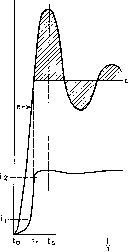

Fig. 243. Non-linear load voltage and current pulse shapes.

voltage E is given in Fig. 244, the ordinates of which are (T de/E)/dt, with E corresponding to the Ea of Fig. 230. Ordinates of Fig. 244 are multiplied by C2E/T to find the initial load current.

Few non-linear loads have absolutely zero current up to the time that voltage E is reached, and the foregoing assumptions are thus

0 0.1 0.2 0.3 0.4 0.5 0,6 0.7 08 0.9

Fig. 244. Front-edge slope of pulse transfoiiiier.

approximate. In spite of this, the following procedure gives fair accuracy.

(a) Find the initial capacitance current as just outlined.

(b) Estimate the current at which the load e-i ешче departs from a straight line {ii, in Fig. 243).

(c) Add currents (a) and (b). This gives 2 (Fig. 243), as the total initial current.

Pulse current continues to rise beyond the value if the initial current value just found is less than the final operating current corresponding to the voltage E: it will droop if the initial current is higher than

the load current at voltage E. To obtain constant current over the greater part of the pulse width, {2 should equal the load current at voltage E. When this equality does not exist, the rate of rise or droop is determined by transformer leakage inductance, source impedance, and load resistance. Where the mode of operation depends upon the rate of voltage rise, as it does in some magnetrons, the initial current may drop off to nearly zero before the main current pulse starts. When there is neghgible initial current ц, the condition for a good current

pulse is E/i2 Л/Е^/С2, where Lg is the leakage inductance.

At the end of the pulse, when the source voltage is reduced to zero (point b, Fig. 226), the circuit reverts to that shown on Fig. 235, but the transformer loses all the load except its own losses. Since by this time it has drawn exciting current, the higher values of Д in the back-swing curves apply. Backswing amplitudes with non-linear loads are complicated and can be predicted only approximately. A procedure for line-type pulsers is given in Chapter 11.

134. Design of Pulse Transformers. [A] Requirements. The performance of a pulse transformer is usually specified by the following:

ia) Pulse voltage. (/) Slope of front,

(b) Voltage ratio. ig) Droop on top.

ie) Pulse duration. {h) Amount of backswing

[d) Repetition rate. permissible.

(e) Power or impedance level. {D Type of load.

Design data ior insuring that these requirements are met are provided in the foregoing sections, in several sets of curves. Below are outlined the steps followed in utilizing these curves for design purposes.

{B) Start of Design. The first step in beginning a design is to choose a core. It is helpful if some previous design exists which is close in rating to the transformer about to be designed.

After choosing the core to be used, the designer must next figure the number of turns. In pulse transformers intended for high voltages, the limiting factor is usually flux density. If so, the number of turns may be derived as follows, for unidirectional pulses:

Ndф , dB

e --X 10-* = NA, - X 10-*

di dt

fe dt = NA.JdB X 10-* (138)

318 ELECTRONIC TRANSFORMERS AND CIRCUITS

For a square wave, e = E and

Er = NArB X 10-

Et X 10*

TV =- (139)

QA5BAc

where E = pulse voltage

t = pulse duration in seconds В = allowable flux density in gauss Ac = core section in square inches N = number of turns.

In many designs, the amount of droop or the backswing which can be tolerated at the end of the pulse determines the munber of turns, because of their relation to the OCL of the transformer.

After the turns are determined, appropriate winding interleaving should be estimated and the leakage inductance and capacitance calculated.

With the leakage inductance and winding capacitance estimated, the front-end performance for linear loads can be found from Figs. 230 and 231. Likewise, from OCL and winding capacitance, the shapes of the top and trailing edge are found in Figs. 234 and 235,. If performance from these curves is satisfactory and the coil fits the core, the design is completed.

(C) Final Calculations. Preliminary calculations may show too much slope on the front edge of the pulse (as often happens with new designs). Two damping factors Rt/2Ls and 1/222 contribute to the front-edge slope, and the prehminary calculations show which one is preponderant. Sometimes it is possible to increase leakage inductance or capacitance without increasing time constant T greatly, and this may be utihzed in decreasing the slope.

If the front-edge slope is still too much after these adjustments, the core chosen is probably inadequate. Small core dimensions are desirable for low leakage inductance and winding capacitance. Small core area Ac may require too many turns to fit the core. These two considerations work against each other, so that the right choice of core is a problem in any design.

If the calculated front-edge slope is nearly good enough it may be improved b one of the following means:

(a) Change number of turns. (d) Increase insulation thickness.

(b) Reduce core size. (e) Reduce insulation dielectric

(c) Change interleaving. constant.

High capacitance is a common cause of poor performance and items (b) to (e) may often be changed to decrease the capacitance. It is sometimes possible to rearrange the circuit to better advantage and thereby make a deficient transformer acceptable. One illustration of this is the termination of a transmission line. Line termination resistance may be placed either on the primary or secondary side. If it is placed on the primary side there is usually a much improved front edge. Figure 231 does not show this improvement inasmuch as it was plotted for Fig. 229. For resistance on the primary side, the damping factor reduces to the single term

R1R2

a =--- (140)

2{Ri + R2)L,

Improvement of the trailing-edge performance usually accompanies improvement of the front edge.

Core permeability is important because it requires fewer turns to obtain the necessary OCL with high-permeability core material. Permeability at the beginning of the trailing edge (point 6, Fig. 236) is most important, for two reasons: the droop at this point depends on the OCL, so that for a given amount of droop the turns on the core are fixed; also, the normal permeability data apply to such points as b\ Flux density is chosen with two aims: it should be as high as possible for small size, but not so high as to result in excessive magnetizing current and backswing voltage.

(D) Example. Assume that the performance requirements are:

Pulse voltage ratio 2,000:10,000 volts. Pulse duration 2 microseconds. Pulse repetition rate 1,000 per second. Impedance ratio 50:1,250 ohms (linear).

To rise to 90 per cent of final voltage in 3 microsecond or less. Droop not to exceed 10 per cent in 2 microseconds. Backswing ampHtude not to exceed 60 per cent of pulse voltage. 50-ohm source.

The final design has the following:

Primary turns = 20. Secondary turns =100.

550 X 10

= 0.18

and from the curve Ri = R2 in Fig. 234, the top droops 9 i)er cent. The magnetizing current is

{Rl -b R2)/R\ X 9 per cent or 18 per cent of the load current

For the backswing

T = 6.28 X 10 л/550 > 00018 = 6 microseconds к = 5.2

From Fig. 235, the backswing is 20 per cent of Ea- If the load resistance is connected to the transformer when the pulse voltage is removed, the backswing superposed oscillation has the same к (1.08) as the front edge, that is, there is no oscillation and the total backswing voltage is 20 per cent of E.

Suppose the load were non-linear; the voltage would rise up to E within %Т or 0.094 microsecond. The front edge

Core: 2-mil silicon steel with 1-mil gap per leg.

Core area = 0.55 sq in.

Core length = 6.3 in. (yh = 0.0003).

Core weight 0.75 lb, window Ц in. X Bie in.

Primary leakage inductance = 2 microhenrys.

Effective primary capacitance = 1,800 f.

No-load loss equivalent to 400 ohms (referred to primary).

, , 10,000 X 2 X 102

Flux density = eT5lO001) :55 =

At 2 microseconds and В = 5,600 ц - 600.

nrt 3.2 X 400 X 0.55 X 10 ,

Primary OCL = - o50 h.

Front-edge performance is figured as follows: K, I SOX 106

21:. + 2й;с. = 4- + 0 =

T = 6.28 X 10- \/2 X О.ООГВ = 0.375 miciosecoiid к = 1.08

According to Fig. 231, this value of к gives 90 per cent of Ea in 0.35Г or 0.131 microsecond.

The top is figured at

tRi 2 X 50 X 10-

PULSE AND VIDEO TRANSFORMERS 50 X 10 . 10

0.8 X 1.8

= 13.2 X 10

From Fig. 244,

к = 0.8

The secondary effective capacitance is 1,800/25 = 72 jujuf and the initial load current is

de 72 X 0.44 X 10,000 Ji= 0.375 X 10 ~ -

Final load current is 10,000/1,250 = 8 amp, and current is non-uniform during the pulse. The backswing is calculated in Chapter 11,

Secondary current is 8 amp. The rms value of this current is, from Table I (p. 16),

/rrae = 8\/20хТ;000 = 0.36 amp

and the primary current is 5 X 0.36 = 1.8 amp. The wire insulation must withstand 10,000 ч- 100 = 100 volts per turn, and with single-layer windings this normally requires at least 0.0014 in. of covering insulation. Heavy enamel wire, No. 28, has a margin of insulation over this value. This is further modified by the initial non-uniform voltage distribution as figured below. A sectional view of a two-coil design is shown in Fig. 245, with No. 28 heavy enamel wire

TO SECONDARY LEAD HV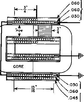

MICA

TO PULSE SOURCE

>MICA

Fig. 245. Section of pulse transformer.