One distributjon law is the Maxwell-Boltzmann probability function. In this case, the particles are considered to be distinguishable by being numbered, for example, from 1 to iV, with no Umit to the number of particles allowed in each energy state. The behavior of gas molecules in a container at fairly low pressure is an example of this distribution.

A second distribution law is the Bose-Einstein function. The particles in this case are indistinguishable and, again, there is no limit to the number of particles permitted in each quantum state. The behavior of photons, or black body radiation, is an example of this law.

The third distribution law is the Fermi-Dirac probability function. In this case, the particles are again indistinguishable, but now only one particle is permitted in each quantum state. Electrons in a crystal obey this law. In each case, the particles are assumed to be noninteracting.

3.5.2 The Fermi-Dirac Probability Function

Figure 3.26 shows the hh energy level with gt quantum states. A maximum of one particle is allowed in each quantum state by the Pauli exclusion principle. There are gi ways of choosing where to place the first particle, (gj - I) ways of choosing where to place the second particle, (g, - 2) ways of choosing where to place the third particle, and so on. Then the total number of ways of arranging Л^ particles in the /th energy level (where Nf < gj) is

(3.76)

Vtis expression includes all permutations of the Nj particles among themselves.

However, since the particles are indistinguishable, the Ni! number of permutations that the particles have among themselves in any given arrangement do not count as separate arrangements. The interchange of any two electrons, for example, does not produce a new arrangement. Therefore, the actual number of independent ways of realizing a distribution of Ni particles in the rth level is

(3.77)

Quantum states

Figure 3-261 The hh energy level with g. quantum states.

EXAMPLE 3.4

Objective

To determine the possible number of ways of realizing a particular distribution. Let g- = 10. Then (g. - ;V,)! = 1.

Solution

Eqization (377) becomes

- - 1

Ni\{gi-N;)\ 10!

Comment

If we have 10 particles to be arranged in 10 quantum states, there is only one possible arrangement. Each quantum state contains one particle.

EXAMPLE 3.5

Objective

To again determine the possible number of ways of realizing a particular distribution. Let gj= 10 and iV. = 9. In this case g -N=\ so that {g - Nf)\ = 1.

Solution

Equation (3.77) becomes

NKg-NiV. (9!)(1)

Comment

In this case, if we have 10 quantum states and 9 particles, there is one empty quantum state. There are 10 possible arrangements, or positions, for the one empty state.

Equation (3.77) gives the number of independent ways of realizing a distribution of Nf particles in the iih level. The total number of ways of arranging (N, Л^з,. , N) indistinguishable particles among n energy levels is the product of all distributions, or

fjNiKg,-Ni)\

(3.78)

The parameter W is the total number of ways in which Л^ electrons can be arranged in this system, where - Li is the total number of electrons in the system. We want to find the most probable distribution, which means that we want to find the maximum W. The maximum W is found by varying Nj among the £, levels, which varies the distriburion, but at the same time, we will keep the total number of particles and total energy constant.

Wc may write the most probable distribution function as

(3.79)

where £f is called the Fermi energy. The number density N{E) is the number of particles per unit volume per unit energy and the function g(E) is the number of quantum states per unit volume per unit energy. The function ff{E) is called the Fermi-Dirac distribution or probability function and gives the probability that a quantum state at the energy E will be occupied by an electron. Another interpretation of the distribution function is that r(£) is the ratio of filled to total quantum states at any energy E,

3.5.3 The Distribution Function and the Fermi Energy

To begin to understand the meaning of the distribution function and the Fermi energy, we can plot the distribution function versus energy. Initially, let Г - 0 К and consider the case when E < Ef. The exponential term in Equation (3.79) becomes exp[(£ - Ef)/kT\ exp i-oo) - 0. The resulting distribution function is ff{E < Ef) = 1. Again let Г = 0 К and consider the case when E > E. The exponential term in the distribution function becomes exp[(E - Ef)/кТ] exp (+oo) +00. The resulting Fermi-Dirac distribution function now becomes ff(E > Ef) - 0.

The Fermi-Dirac distribution function for Г - 0 К is plotted in Figure 3.27. This result shows that, for Г 0 K, the electrons are in their lowest possible energy states. The probability of a quantum state being occupied is unity for £ < Ef and the probability of a state being occupied is zero for £ > Ef. All electrons have energies below the Fermi energy at T - 0 K.

Figure 3.28 shows discrete energy levels of a particular system as well as the number of available quantum states al each energy. If we assume, for this case, that

5 1,0

Figure 3.27 1 The Fermi probability function versus energy for Г - 0 K.

UUVJUUUUUU

www www

WW WW

Figure 3.28 I Discrete energy states and quantum states for a particular system at T = 0 K.

the system contains 13 electrons, then Figure 3,28 shows how these electrons are distributed among the various quantum states at Г = 0 K. The electrons will be in the lowest possible energy state, so the probability of a quantum state being occupied in energy levels Ei through E4 is unity, and the probability of a quantum state being occupied in energy level E5 is zero. The Fermi energy, for this case, must be above £4 but less than £5. The Fermi energy determines the statistical distribution of electrons and does not have to correspond to an allowed energy level.

Now consider a case in which the density of quantum states g(E) is a continuous function of energy as shown in Figure 3.29. If we have Nq electrons in this system, then the distribution of these electrons among the quantum states at Г = 0 К is shown by the dashed line. The electrons are in the lowest possible energy state so that all states below Ef. are filled and all states above Ef are empty. If and Nq are known for this particular system, then the Fermi energy Ef can be determined.

Consider the situation when the temperature increases above T = 0 K, Electrons gain a certain amount of thermal energy so that some electrons can jump to higher energy levels, which means that the distribution of electrons among the available energy states will change. Figure 3.30 shows the same discrete energy levels and quantum states as in Figure 3.28. The distribution of electrons among the quantum states has changed from the Г - 0 К case. Two electrons from the £4 level have, gained enough energy to jump to £5, and one electron from £3 has jumped to £4. As the temperature changes, the distribution of electrons versus energy changes.

The change in the electron distribution among energy levels for Г > 0 К can be seen by plotting the Fermi-Dirac distriburion function. If we let E = Ep and Г > OK, then Equation (3.79) becomes

ME = Ef) -

l+exp(0) 1-h I

The probability of a state being occupied at E - Ef is . Figure 3.31 shows thej Fermi-Dirac distribution function plotted for several temperatures, assuming the Fermi energy is independent of temperature.

g{E) dE

\JVJVJ\VJW\JVJVJ

Figure 3.291 Density of quantum states and electrons in a continuous energy system at Г = 0 K.

Figure 3.301 Discrete energy states and quantum states for the same system shown in Figure 3.28 for Г > OK.

7- 0

Figure 3.31 f The Fermi probability function versus energy for different temperatures.

We can see that for temperatures above absolute zero, there is a nonzero probability that some energy states above Ef will be occupied by electrons and some energy states below Ef will be empty. This result again means that some electrons have jumped to higher energy levels with increasing thermal energy.

Objective

To calculate the probability that an energy state above Ef is occupied by an electron.

Let T = 300 K. Determine the probability that an energy level 3/:T above the Fermi energy is occupied by an electron.

Solution

From Equation (3.79), we can write

EXAMPLE 3.6

fFiE) =

1 + exp 1

ПкТ

which becomes

ff{E) =

T + 20.09

= 0.0474 = 4.74%

Comment

At energies above Ef., the probability of a state being occupied by an electron can become significantly less than unity, or the ran о of electrons to available quantum states can be quite small.

TEST YOUR UNDERSTANDING

E34 Assume the Fermi energy level is 0.30 eV below the conduction band energy-Co) Determine the probability of a stale being occupied by an electron at E.. ф) Repeat part (a) for an energy state at -h /: T. Assume T = 300 K. U-Ol X £f e (Я) 4 01 X zee () suvl

EXAMPLE 3.7

E3.5 Assume the Fermi energy level is 0.35 eV above the valence band energy.

(a) Determine the probability of a state being empty of an electron at E. {b) Repeat part (a) for an energy state at Ev - кТ. Assume T = 300 K.

[-01 X s6 №'9-oi X еет о^)* чу]

We can see from Figure 3.31 that the probability of an energy above £> bein occupied increases as the temperature increases and the probability of a state belov Ef being empty increases as the temperature increases.

Objective

To determine the temperature at which there is a 1 percent probability that an energy state empty.

Assume that the Fermi energy level for a particular material is 6.25 eV and that the electrons in this material follow the Fermi-Dirac distribution function. Calculate the temperatun at which there is a I percent probability that a slate 0.30 eV below the Fermi energy level wij not contain an electron.

Solution

The probability that a state is empty is

\-fAE) = }--

1 H-exp

Then

0.01 = 1 -

1 + exp

5.95-6

Solving for AT, we find кТ = 0.06529 eV, so that the temperature is T 756 K.

Comment

The Ferini probability function is a strong function of temperature.

TEST YOUR UNDERSTANDING

E3.6 Repeat Exercise E3.4 for T = 400 K. 1 g-0\ x 0Z*9 (*?) Ч-01 x 69 I ( ) *иу] E3.7 Repeat Exercise E3.5 for T = 400 K. [ -01 x 9V\ W 4-01 x %e 0 Vl

We may note that the probability of a state a distance dE above Ef Ыщ occupied is the same as the probability of a state a distance dE below Ef heh empty. The function ff(E) is symmetrical with the function 1 - ffiE) about Fenni energy, Ef. This symmetry effect is shown in Figure 3.32 and will be u! in the next chapter.

ME) [ -f,(E)

Figure 3.32 I The probabihty of a state being occupied,

and the probabihty of a state being empty, I - ./>{£).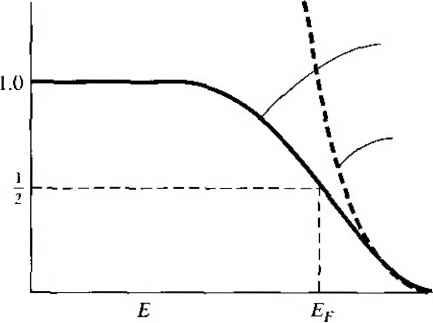

Fermi-Dirac tunciion

Boltzmann approximation

Figure 3.33 1 The Fermi-Dirac probability function and the Maxwell-Boltzmann approximation.

Consider the case when E - Ef кТ. where the exponential term in the denominator of Equation (ЗЛ9) is much greater than unity. We may neglect the 1 in the denominator, so the Fermi-Dirac distribution function becomes

ffiE) exp

(3.80)

Equation (3.80) is known as the Maxwell-Boltzmann approximation, or simply the Bo)t2mann approximation, to the Fermi-Dirac distribution function. Figure 3,33 shows the Fermi-Dirac probability function and the Boltzmann approximation. This figure gives an indication of the range of energies over which the approximation is valid.

Objective

To determine the energy at which the Boltzmann approximation may be considered valid.

Calculate the energy, in terms of AT and Ef. at which the difference between the Boltzmann approximafion and the Fermi-Dirac function is 5 percent of the Fermi function.

EXAMPLE 3.8

Solution

We can write

[ кТ

I + exp

E - E кТ

- 0.05

1 + exp

If we multiply both numerator and denominator by the 1 + exp () function, we have

- I - 0.05

which becomes

-{EEf)

= 0.05

(E- Er)kT In

V0.05

ЪкТ

m Comment

As seen in this example and in Figure 3.33, the E - Et кТ notation is somewhat misleading. The Maxwell-Boltzmann and Fermi-Dirac functions are within 5 percent of each i>ther when E - Ef ЪкТ.

The actual Boltzmann approximation is valid when exp[(E - Et)/kT] 1. However, it is stil! common practice to use the E - Ef кТ notation when applying the Boltzmann approximation. We will use this Boltzmann approxiiuation in our discussion of semiconductors in the next chapter.

3.6 I SUMMARY

Discrete allowed electron energies split into a band of allowed energies as atoms are brought together to form a crystal.

Ш The concept of allowed and forbidden energy bands was developed more rigorously by considering quantum mechanics and Schrodinger *s wave equation using the Kronig-Penney model representing the potential function of a single crystal material. This result forms the basis of the energy band theory of semiconductors.

The concept of effective mass was developed. Effective mass relates the motion of a particle in a crystal to an externally applied force and takes into account the effect of the crystal lauice on the motion of the particle,

Ш Two charged particles exist in a semiconductor. An electron is a negatively charged particle with a positive effective mass existing at the bottom of an allowed energy band. A hole is a positively charged particle with a positive effective mass existing at the top of an allowed energy band.

Checkpoint 97

The E versus k diagram of silicon and gallium arsenide were given and the concept of direct and indirect bandgap semiconductors was discussed.

Energies within an allowed energy band are actually at discrete levels and each contains a finite number of quantum states. The density per unit energy of quantum states was determined by using the three-dimensional infinite potential well as a model. In dealing with large numbers of electrons and holes, we must consider the statistical behavior of these particles. The Fermi-Dirac probability function was developed, which gives the probability of a quantum state at an energy E of being occupied by an electron. The Fermi energy was defined.

GLOSSARY OF IMPORTANT TERMS

allowed energy band A band or range of energy levels that an electron in a crystal is allowed to occupy based on quantum mechanics.

density of states function The density of available quantum states as a function of energy, given in units of number per unit energy per unit volume.

electron effective mass The parameter that relates the acceleration of an electron in the conduction band of a crystal to an external force; a parameter that takes into account the effect of internal forces in the crystal.

Fermi-Dirac probability function The function describing the statistical distribution of electrons among available energy states and the probability that an allowed energy state is occupied by an electron.

fermi energy In the simplest definifion, the energy below which all states are filled with electrons and above which all states are empty at Г = 0 K.

forbidden energy band A band or range of energy levels that an electron in a crystal is not allowed to occupy based on quantum mechanics.

hole The posifively charged particle associated with an empty state in the top of the valence band.

hole effective mass The parameter that relates the acceleration of a hole in the valence band of a crystal to an applied external force (a positive quantity); a parameter that takes into account the effect of intemal forces in a crystal.

Jt-space diagram The plot of electron energy in a crystal versus k, where к is the momentum-related constant of the motion that incoфorates the crystal interaction.

Kronig-Penney model The mathemafical model of a periodic potential funcnon representing a one-dimensional single-crystal lattice by a series of periodic step funcfions.

Maxwell-Boltzmann approximation The condifion in which the energy is several кТ above the Fermi energy or several кТ below the Fermi energy so that the Fermi-Dirac probability function can be approximated by a simple exponential function.

Pauli exclusion principle The principle which states that no two electrons can occupy the same quantum state.

CHECKPOINT

After studying this chapter, the reader should have the abifity to:

Discuss the concept of allowed and forbidden energy bands in a single crystal both qualitafively and more rigorously from the results of using the Kronig-Penney model.

CHAPTERS IntroductiontotheQuantumTheoryofSolids

Discuss the sphtting of energy bands in sihcon.

State the definition of effective mass from the E versus k diagram and discuss its meaning in terms of the movement of a particle in a crystal. Discuss the concept of a hole.

Qualitatively, in terms of energy bands, discuss the difference between a metal,

insulator, and semiconductor

Discuss the effective density of states function.

Understand the meaning of the Fermi-Dirac distribution function and the Fenni energy.

REVIEW QUESTIONS

2. 3. 4. 5. 6. 7. 8. 9.

What is the Kronig-Penney model?

State two results of using the Kronig-Penney model with Schrodingers wave equation. What is effective mass?

What is a direct bandgap semiconductor? What is an indirect bandgap semiconductor? What is the meaning of the density of states function?

What was the mathematical model used in deriving the density of states function? In general, what is the relation between density of states and energy? What is the meaning of the Fermi-Dirac probability function? What is the Fermi energy?

PROBLEMS

3.5

о

Section ЗЛ Allowed and Forbidden Energy Bands

3.1 Consider Figure 3.4b, which shows the energy-band splitting of silicon. If the

equihbrium lattice spacing were to change by a small amount, discuss how you would expect the electrical properties of silicon to change. Determine at what point the material would behave like an insulator or like a metal.

Show that Equations (3.4) and (3.6) are derived from Schrodingers wave equation, using the form of solution given by Equation (3.3).

Show that Equations (3.9) and (3.10) are solutions of the differential equations given by Equations (3.4) and (3.8), respectively.

Show that Equations (3.12), (3.14), (3.16), and (3.18) result from the boundary conditions in the Kronig-Penney model.

Plot the function /{aa) - 9\naa/aa + cosa for 0 <aa < 6я. Also, given the function f{aa) - cos ka, indicate the allowed values of aa which will satisfy this equation.

3.6 Repeat Problem 3.5 for the function

f{aa) = 6sinaa/aa -{-cosaa - cos ka

3.7 Using Equation (3.24), show that dE/dk = 0 mtk = nnja, where n = 0, 1, 2.....

3.8 Using the parameters in Problem 3.5 and letting a -ЪК, determine the width (in eV) of the forbidden energy bands that exist at (л) ka = {b) ka = 2л, (с) = Зтг, and {d)ka Refer to Figure 3.8c.