tinPp(p-n)

Equation (6.39) is cailed the ambipolar transport equation and describes the behavior of the excess electrons and holes in time and space. The parameter D is called the ambipolar diffusion coefficient and is called the ambipolar mobility.

The Einstein relation relates the mobility and diffusion coefficient by

(6.42)

Using these relations, the ambipolar diffusion coefficient may be written in the form

ОпП + Dpp

(6.43)

The ambipolar diffusion coefficient, D\ and the ambipolar mobility, p\ are functions of the electron and hole concentrations, n and p, respectively. Since both n and p contain the excess-carrier concentration 5п, the coefficient in the ambipolar transport equation are not constants. The ambipolar transport equation, given by Equation (6.39), then, is a nonlinear differential equation.

6 J.2 Limits of Extrinsic Doping and Low Injection

The ambipolar transport equation may be simplified and linearized by considering an extrinsic semiconductor and by considering low-level injection. The ambipolar diffusion coefficient, from Equation (6.43), may be written as

DnDp[{m8n) + {po + 8n)] T>,Mo + <5rt) Ч- Dpipo + Sn)

(6,44)

where о and p are the thermal-equilibrium electron and hole concentrations, respectively, and bn\s the excess carrier concentration. If we consider a p-type semiconductor, we can assume that po o- The condition of low-leverinjection, or just low injection, means that the excess carrier concentration is much smaller than the thermal-equilibrium majority carrier concentration. For the p-type semiconductor, then, low injection implies that Sn <K po Assuming that л о <§C po and Sn <K po, and assuming that Д, and Dp are on the same order of magnitude, the ambipolar diffusion coefficient from Equation (6.44) reduces to

D = On (6.45)

If we apply the conditions of an extrinsic p-type semiconductor and low injection to the ambipolar mobility, Equation (6.41) reduces to *

L;, It is important to note that for an extrinsic p-type semiconductor under low mnjection, the ambipolar diffusion coefficient and the ambipolar mobility coefficient reduce to the minority-carrier electron parameter values, which are constants. The ambipolar transport equation reduces to a linear differential equation with constant coefficients.

If we now consider an extrinsic n-type semiconductor under low injection, we may assume that po o and 5/? о* The ambipolar diffusion coefficient from Equation (6.43) reduces to

=- Dp (6.47)

and the ambipolar mobility from Equation (6.41) reduces to

- -M, (6.48)

ambipolar parameters again reduce to the minority-carrier values, which are constants. Note that, for the n-type semiconductor, the ambipolar mobility is a negative value. The ambipolar mobility tenti is associated with cairier drift; therefore, the sign of the drift term depends on the charge of the particle. The equivalent ambipolar particle is negatively charged, as one can see by comparing Equations (6.30) and (6.39). If the ambipolar mobility reduces to that of a positively charged hole, a negative sign is introduced as shown in Equation (6.48).

The remaining terms we need to consider in the ambipolar transport equation are the generation rate and the recombination rate. Recall that the electron and hole recombination rates are equal and were given by Equation (635) as - n/int - р/Тр( = R, where т„ and are the mean electron and hole Ufetimes, respectively. If we consider the inverse lifetime functions, then 1 /т„г is the probability per unit time that an electron will encounter a hole and recombine. Likewise, l/Tpf is the probability per unit rime that a hole will encounter an electron and recombine. If we again consider an extrinsic p-type semiconductor under low injection, the concentration of majority carrier holes will be essentially constant, even when excess carriers are present. Then, the probability per unit time of a minority carrier electron encountering a majority carrier hole will be essentially constant. Hence т„, = r , the minority carrier electron lifetime, will remain a constant fV)r the extrinsic p-type semiconductor under low injection.

Similarly, if we consider an extrinsic n-type semiconductor under low injection, the minority carrier hoie lifetime, Vpt r will remain constant. Even under the condition of low injection, the minority carrier hole concentration may increase by several orders of inagnitude. The probability per unit lime of a majority carrier electron encountering a hole may change drastically. The majority carrier lifetime, then, may change substantially when excess carriers arc present.

Consider, again, the generation and recombination terms in the ambipolar transport equation. For electrons we may write

g-R=.g,-R,= (G o + gj - + О (6.49)

where С„о and g, are the thermal-equilibrium electron and excess electron generation rates, respectively. The terms Rf,o and R are the thermal-equilibrium electron

and excess electron recombination rates, respectively. For thermal equilibrium, we have that

G o - R

(6.50)

so Equation (6.49) reduces to

(6.51)

where т„ is the excess minority carrier electron lifetime. For the case of holes, we may write

(6.52)

g-gp-p iGpo+gp) - {Rpiy + /?;)

where Gpo and g are the thermal-equilibrium hole and excess hole generation rates, respectively. The terms Rpo and R are the thermal-equilibrium hole and excess hole recombination rates, respectively. Again, for thermal equilibrium, we have that

(6.53)

so that Equation (6.52) reduces to

(6.54)

where is the excess minority carrier hole lifetime.

The generation rate for excess electrons must equal the generation rate for excess holes. We may then define a generation rate for excess carriers as g\ so that gn - gp = g determined that the minority carrier lifetime is essentially a

constant for low injection. Then the term g - R in the ambipolar transport equation may be written in terms of the minority-carrier parameters.

The ambipolar transport equation, given by Equation (6.39), for a p-type semiconductor under low injection then becomes

(6.55)

The parameter 8n is the excess minority carrier electron concentration, the parameter r o is the minority carrier lifetime under low injection, and the other parameters are the usual minority carrier electron parameters.

Similarly, for an extrinsic n-type semiconductor under low injection, the ambipolar transport equation becomes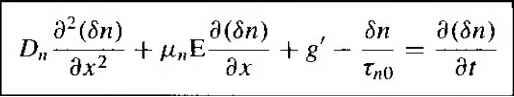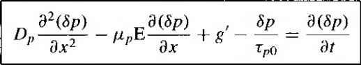

(6.56)

The parameter 5/? is the excess minority carrier hole concentration, the parameter т^о is the minority carrier hole lifetime under low injection, and the other parameters are the usual minority carrier hole parameters.

Table 6,2 I Common ambipolar transport equation simplifications

Specification

Effect

Steady state

Uniform distribution of excess carriers (uniform generation rate)

Zero electric field

No excess carrier generation

No excess carrier recombination (infinite lifefime)

d{Sn) d{5p)

a(5 )

E-=0. E-=0 dx dx

Sn Sp - =0, - = 0 Гдп r,o

It is extremely important to note that the transport and recombination parameters in Equations (6.55) and (6.56) are those of the minority carrier. Equations (6.55) and describe the drift, diffusion, and recombination of excess minority carriers as a function of spatial coordinates and as a function of time. Recall that we had imposed the condition of charge neutrality; the excess minority carrier concentration is equal to the excess majority carrier concentration. The excess majority carriers, then, diffuse and drift with the excess minority carriers; thus, the behavior of the excess majority carrier is determined by the minority carrier parameters. This ambipolar phenomenon is extremely important in semiconductor physics, and is the basis for describing the characteristics and behavior of semiconductor devices.

6.3.3 Applications of the Ambipolar Transport Equation

We will solve the ambipolar transport equation for several problems. These examples will help illustrate the behavior of excess carriers in a semiconductor material, and the results will be used later in the discussion of the pn junction and the other semiconductor devices.

The following examples use several common simplifications in the solution of the ambipolar transport equation. Table 6.2 summarizes these simplificarions and their effects.

Objective

To determine the time behavior of excess carriers as a semiconductor returns to thennal equilibrium.

Consider an infinitely large, homogeneous n-type semiconductor with zero applied electric field. Assume that at time f = 0, a uniform concentration of excess carriers exists in the crystal, but assume that g =0 for Г > 0. If we assume that the concentration of excess carriers is much smaller than the thermal-equilibrium electron concentration, then the low-injeclion condition applies. Calculate the excess carrier concentration as a function of time for t > 0.

EXAMPLE 6.1

Solution

For ttie n-type semiconductor, we need to consider the ambipolar transport equation for the minority carrier holes, which was given by Equation (6,56), The equation is

dHsp) шр) , Sp d(Sp)

Or,-.--PpB + g ~

We are assuming a uniform concentration of excess holes so that d(Sp)/Bx = 3 (Sp)/Bx = 0. For r > 0, we are also assuming that g ~ 0. Equation (6.56) reduces to

diSp) Sp

(6.57)

Since there is no spatial variation, the total time derivative may be used. At low injection, the minority carrier hole lifetime, Zpo, is a constant. The solution to Equation (6.57) is

Spit) = Sp(0)e-p

(6.58)

where Sp{0) is the uniform concentration of excess carriers that exists at time f = 0. The concentration of excess holes decays exponentially with time, with a time constant equal to the minority carrier hole lifetime.

From the charge-neutrality condition, we have that Sn = Sp, so the excess electron concentration is given by

Snit) = Sp(0)e-p

(6.59)

Numerical Calculation

Consider n-type gallium arsenide doped at = lO cm~. Assume that 10 electron-hole pairs per cm have been created at f = 0, and assume the minority carrier hole lifetime is Tpo = 10 ns.

We may note that Sp{0) <$C о. so low injection applies. Then from Equation (6.58) we can write

5p(0 = 10V cm-

The excess hole and excess electron concentrations will decay to 1 /e of their initial value in 10 ns.

Comment

The excess electrons and holes recombine at the rate determined by the excess minority carrier hole lifetime in the n-type semiconductor.

EXAMPLE 6.2

Objective

To determine the time dependence of excess carriers in reaching a steady-state condition.

Again consider an infinitely large, homogeneous n-type semiconductor with a zero applied electric field. Assume that, for t < 0, the semiconductor is in thermal equilibrium and

, 8p djSp) Tpo ~ dt

The solution to this differential equation is

(6.60)

Sp{t) = gTpo(\-e-)

(6.61)

Numerical Calculation

Consider n-type silicon at T = 300 К doped at A = 2x 10 cm. Assume that Г/,о = 10 s and = 5 X 10 cm~- s~. From Equation (6.61) we can write

Spit) = (5 X 10- )(10-)Г1 - e-1 = 5 X 10 [l - e

Comment

We may note that for / -> oo, we will create a steady-state excess hole and electron concentration of 5 X 10 cm~-. We may note that dp <SC hq, so low injection is valid.

The excess minority carrier hole concentration increases with time with the same time constant Zpo, which is the excess minority carrier lifetime. The excess carrier concentration reaches a steady-state value as time goes to infinity, even though a steady-state generation of excess electrons and holes exists. This steady-state effect can be seen from Equation (6.60) by scitmg d{Sp)/dt - 0. The remaining tenns simply state that, in steady state, the generation rate is equal to the recombination rate.

TEST YOUR UNDERSTANDING

E6.3 Silicon at 7 = 300 К has been doped with boron atoms to a concentration of

ТУд = 5 X 10 cm -\ Excess carriers have been generated in the uniformly doped material to a concentration of lO* cm~. The minority carrier lifetime is 5 s, (a) What carrier type is the minority carrier? (b) Assuming g = F = 0 for / > 0, determine the minority carrier concentration for / > 0. [, шэ xy/.-siOl (Я) suojpap (V) suvl

E6.4 Consider silicon with the same parameters as given in E6.3. The material is in

thermal equilibrium for t < 0. At / = 0, a source generating excess carriers is turned on, producing a generation rate of g = 10* cm~ -s . (a) What carrier type is the minority carrier? {b) Determine the minority carrier concentration for / > 0. (c) What is the minority carrier concentration as r -oo?

[с-шо ,01 X g (э) V- mD [01x5/1- - llOI x 5 (Ф suojoia (r?) suy]

that, for / > 0, a uniform generation rate exists in the crystal. Calculate the excess carrier concentration as a function of time assuming the condition of low injection.

Solution

The condition of a uniform generation rate and a homogeneous semiconductor again imphes that д^{Ьр)1дх = д{8р)/дх = 0 in Equation (6.56). The equation, for this case, reduces to

EXAMPLE 6.3

Objective

To determine the steady-state spatial dependence of the excess carrier concentration.

Consider a p-type semiconductor that is homogeneous and infinite in extent. Assume a zero applied electric field. For a one-dimensional crystal, assume that excess carriers are being generated at j: = 0 only, as indicated in Figure 6.6. The excess carriers being generated at X = 0 will begin diffusing in both the +x and -x directions. Calculate the steady-state excess carrier concentration as a function of a-.

Solution

The ambipolar transport equation for excess minority carrier electrons was given by Equation (6,55), and is written as

Sn 3(Sn)

From our assumptions, we have E = 0, = 0 for .v 0, and 3(Sn}/3t = 0 for steady state. Assuming a one-dimensional crystal, Equation (6,55) reduces to

d-{Sn) Sn

(6.62)

Dividing by the diffusion coefficient, Equafion (6.62) may be written as

d{Sn) Sn d-(Sn) Sn

dx Dn T,jQ dx-

(6,63)

where we have defined L\ D,jT o. The parameter L has the unit of length and is called the minority carrier electron diffusion length. The general solufion to Equation (6.63) is

(6.64)

As the minority caiTier electrons diffuse away from jc = 0, they will recombine with the majority carrier holes. The minority carrier elecu-on concentration will then decay toward zero at both -V = +OC andA = -oc. These boundary conditions mean that В 0 for x > 0 and A = 0 for JC < 0. The solution lo Equation (6.63) may then be written as

Sn{x) =SniO)e

X > 0

(6.65a)

x = 0

Figure 6,61 Steady-state generation rate at JC =0.

(6.65b)

where Sn(0} is the value of the excess electron concentration at л = 0. The steady-state excess electron concentration decays exponentially with distance away from the source at

Numerical Calculation

Consider p-type silicon at Г = 300 К doped at =5 x 10*cni~\ Assume that r o ~ 5 X 10- s, Д, = 25 cm/s, and Sn(0} = 10 cm- The minority carrier diffusion length is

En = y/D t,o = /(25)i5Г[0) = 35.4 дт Then for X > 0, we have

Comment

We may note that the steady-state excess concentration decays to l/e of its value at jr = 35.4 дт.

As before, we will assume charge neutrality; thus, the steady-state excess majority carrier hole concentration also decays exponentially with distance with the same characteristic minority carrier electron diffusion length L . Figure 6.7 is a plot of the total electron and hole concentrarions as a function of distance. We are assuming low injection, that is, 5/7(0) < po in the p-type semiconductor. The total concentration of majority carrier holes barely changes. However, we may have Sn(0) no and srill satisfy the low-injecrion condirion. The minority carrier concentration may change by many orders of magnitude.

TEST YOUR UNDERSTANDING

E6.5 Excess electrons and holes are generated at the end of a silicon bar (x =0). The

silicon is doped with phosphorus atoms to a concentration of Nd - 10 cm~-. The minority carrier lifetime is 1 /xs, the electron diffusion coefficient is Dj =25 cm-/s, and the hole diffusion coefficient is Dp 10 cm/s. If 5л(0) = 6p(0) = 10 cm~, determine the steady-state electron and hole concentrations in the silicon for jc > 0.

E6.6 Using the parameters given in E6.5, calculate the electron and hole diffusion current densities atjc = 10 дт. (шэ/у 69e0- = Y \uio/v 69e*0+ = V * ¥)

The three previous examples, which applied the ambipolar transport equation to specific situations, assumed either a homogeneous or a steady-state condirion; only the rime variation or the spatial variation was considered. Now consider an example in which both the time and spatial dependence are considered in the same problem.

Carrier concentration (1оц scale)

Uq + 8пф)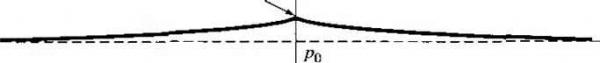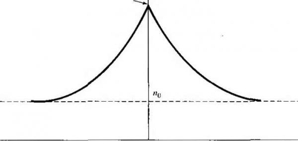

x = 0

Figure 6.7 I Steady-state electron and hole concentrations for the case when excess electrons and holes are generated at л = 0.

EXAMPLE 6.4

Objective

To determine both the dme dependence and spadal dependence of the excess carrier concentration.

Assume that a iinite number of electron-hole pairs is generated instantaneously at time / = 0 and at X = 0, but assume g = 0 for t > 0. Assume we have an n-type semiconductor with a constant applied electric field equal to Eo, which is applied in the -\-x direction. Calculate the excess carrier concentration as a function of x and /.

Solution

The one-dimensional ambipolar transport equation for the minority carrier holes can be written from Equation (6.56) as

SH5p) HSp) 5p d(8p) Dn-.--Д;,Ео

dx V

The solution to this partial differential equation is of the form

<5р(л, r) = p{xj)e-

(6.66J

(6.67)

By substituting Equation (6.67) into Equation (6.66), we are left with the partial differential equation

dp\x,t)

- PpEo

dpixA) dp(xj)

(6.68)

Equation (6.68) is normally solved using Laplace transform techniques. The solution, without going through the mathematical details, is

4D,t

(6.69)

The total solution, from Equations (6.67) and (6,69), for the excess minority carrier hole concentration is

Spix, t) =

-jx - tipEpt) 4D,t

2 -1

(6.70)

Comment

We could show that Equation (6.70) is a solution by direct substitution back into the partial differential equation. Equation (6.66).

Equation (6.70) can be plotted as a function of distance x, for various times. Figure 6.8 shows such a plot for the case when the applied electric field is zero. For > 0, the excess minority carrier holes diffuse in both the T-x and -x directions. During this time, the excess majority carrier electrons, which were generated, diffuse at exactly the same rate as the holes. As time proceeds, the excess holes recombine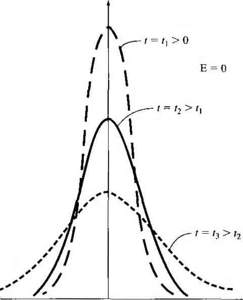

л - 0

Distance, x

Figure 6-81 Excess-hole concentration versus distance at various times for zero applied electric field.