15 -

% 10

(Л

0 = 2

n = 1

jc = 0

л = a

л- = 0

Figure 2.6 1 Particle in an infinite potential well: (a) Four lowest discrete energy levels, (b) Corresponding wave funcdons. (c) Corresponding probability functions, (From Pierret (91)

TEST YOUR UNDERSTANDING

E2.5 The width of the infinite potential well in Example 2,3 is doubled to 10 A. Calculate the first three energy levels in terms of electron volts for an electron. (ЛЭ ЛЭ ogl л^ Ш'О SUV)

E2-6 The lowest energy of a particle in an infinite potential well with a width of 100 A is 0.025 eV. What is the mass of the particle? it-Ol x Ll\ SUV)

2.3.3 The Step Potential Function

Consider now a step potential function as shown in Figure 2.7 .In the previous section, we considered a particle being confined between two potential barriers. In this example, we will assume that a flux of particles is incident on the potential barrier. We will assume that the particles are traveling in the -\-x direction and that they originated at jr = - oo. A particularly interesting result is obtained for the case when the total energy of the particle is less than the barrier height, or £ < Vo-

We again need to consider the time-independent wave equation in each of the two regions. This general equation was given in Equation (2.13) as 9i(.r)/9x+ 2mjf?{E - V{x))l/{x) = 0. The wave equation in region I, in which 1/ = 0, is

diix) 2m E

2-3 AppI ications of Schrod i ngers Wave Equation

x = 0

Figure 2.7 I The step potential function.

The general solution to this equation can be written in the form

ViCv) = A,> + Bie- (x < 0) where the constant K\ is

(2.40)

AT, -

2m E

(2,41)

The first term in Equation (2.40) is a traveling wave in the +x direction that represents the incident wave, and the second term is a traveling wave in the -x direction that represents a reflected wave. As in the case of a free particle, the incident and reflected particles are represented by traveling waves.

For the incident wave, A i - A* is the probability density function of the incident particles. If we muUiply this probability density function by the incident velocity, then Ai Aj is the flux of incident particles in units of #/cm-s. Likewise, the quantity Vr B* is the flux of the reflected particles, where ь\ is the velocity of the reflected wave. (The parameters and Vr in these terms are actually the magnitudes of the velocity only.)

In region II, the potential is V = Vq, If we assume that £ < Vq, then the differential equation describing the wave function in region II can be written as

д'ф->(х) 2m

- tt(Vo - E)2M - 0 (2.42)

The general solution may then be written in the form

Ых) = A2e- + 2 - (x > 0)

where

(2-43)

K2 =

2m(Vo - E)

(2.44)

One boundary condition is that the wave function yj/iix) must remain finite, which means that the coefficient 2 = 0- The wave function is now given by

Ых) = Aje (x > 0) (2.45)

The wave function at x 0 must be continuous so that

i(0)-2(0) Then from Equations (2.40), (2.45), and (2.46), we obtain

Ai+i =A2

(2.46)

(2.47)

Since the potential function is everywhere finite, the first derivative of the wave function must also be continuous so that

(2.48)

Using Equations (2.40), (2.45), and (2.48), we obtain

jKAx - jKBx = -K2A2

(2.49)

We can solve Equations (2.47) and (2.49) to determine the coefficients B\ and A2 in terms of the incident wave coefficient Ai. The results are

5i =

-{Kl + 2jKiK2-K)A, {Ki + K})

2K,(K -jK2)A,

(2.50a)

{i + )

The reflected probability density function is given by

{K- -\-2jKiK2){K; - Kf -2jKiK2)Ai Л

(2.50b)

(2-51)

We can define a reflection coefficient, as the ratio of the reflected flux to the incident flux, which is written as

v\ A\ A*

(2-52)

where tv r are the incident and reflected velocities, respectively, of the particles. In region \,V = Q so that E T, where T is the kinetic energy of the particle. The kinetic energy is given by

T - -mv 2

so that the constant Ai, from Equation (2.41), may be written as

(2.53)

The incident velocity can then be written as

Vi = - (2.55)

Since the reflected particle also exists in region I, the reflected velocity (magnitude) is given by

Vr = -Ki (2.56)

The incident and reflected velocities (magnitudes) are equal. The reflection coefficient is then

Vr B] ВТ B\ ВТ R = = -f-i (2.57)

Substituting the expression from Equation (2.51) into Equation (2.57), we obtain

R = ~-L = w-< 2- J Q 2.58)

The result of R - [ implies that all of the particles incident on the potential barrier for E < Vq arc eventually reflected. Particles are not absorbed or transmitted through the potential barrier. This result is entirely consistent with classical physics and one might ask why we should consider this problem in terms of quantum mechanics. The interesting result is in terms of what happens in region II.

The wave solution in region II was given by Equation (2.45) as ф2 (x) = A 2~--. The coefficient An from Equation (2.47) is a2 = + 1, which we derived from the boundary conditions. For the case ofE < Vq, the coefficient A2 is not zero. If Л2 is not zero, then the probability density function \l/2{x) т (х) of the particle being found in region II is not equal to zero. This result implies that there is a finite pro bability that the incident particle will penetrate the potential barrier and exist in region II. The probability of a particle penetrating the potential barrier is another difference between cla.ssicol and quantum mechanics: The quantum mechanical penetration is classically not allowed. Although there is a finite probability that the particle may penetrate the barrier, since the reflection coefficient in region I is unity, the particle in region II must eventually turn around and move back into region I.

Objective example ia

To calculate the penetration depth of a particle impinging on a potential barrier

Consider an incident electron that is traveting at a velocity of I x 10 m/s in region I.

Solution

With V(x) = 0, the total energy is also equal to the kinetic energy so that

ET = -mv- = 4.56 X 10 J = 2.85 x 10 eV 2

Now, assume that the potential barrier at л =0 is twice as large as the total energy of the incident particle, or that Vo =2E, The wave function solution in region II is t2() = 2~-\ where the constant К2 is given by К2 = 2m(Vo - E)/ff.

In this example, we want to determine the distance x = J at which the wave function magnitude has decayed to of its value at л = 0. Then, for this case, we have Kid = 1 or

,2m(2£ - E) 2mE

The distance is then given by

1.054 X 10

= 11.6 X 10- m

2(9.11 X 10-)(4.56 X 10-21) or

d = 11.6 A

Comment

This penetration distance corresponds to approximately two lattice constants of silicon. The numbers used in this example are rather arbitrary. We used a distance at which the wave function decayed to e~ of its initial value. We could have arbitrarily used e~-, for example, but the results give an indication of the magnitude of penetration depth.

The case when the total energy of a particle, which is incident on the potential barrier, is greater than the barrier height, or £ > Va, is left as an exercise at the end of the chapter.

TEST YOUR UNDERSTANDING

E2.7 The probability of finding a particle al a distance d in region It compared lo that at

X = 0 is given by exp {-2 К 2d). Consider an electron traveling in region I at a velocity of 10 m/s incident on a potential barrier whose height is 3 dmes the kinetic energy of the electron. Find the probability of finding the electron at a distance d

compared to jc = 0 where d is (a) 10 A and {h} 100 A into the potential barrier, [luaojad oi x £4 (q) щ^оЫ zu% (v) *suv]

2,3.4 The Potential Barrier

We now want to consider the potential barrier function, which is shown in Figure 2.8. The more interesting problem, again, is in the case when the total energy of an incident particle is E < Vo- Again assume that we have a flux of incident particles originating on the negative x axis traveling in the -\-x direction. As before, we need to solve Schrodingers time-independent wave equation in each of the three regions. The

V(x)

Л- - a

Figure 2.81 The potential barrier function.

solutions of the wave equation in regions I, II, and III are given, respectively, as

(2.59a) (2.59b)

(2.59c)

where

2m E

(2.6Qa)

(Vo - E)

(2.60b)

The coefficient in Equation (2.59c) represents a negative traveling wave in region HI. However, once a particle gets into region III, there are no potential changes to cause a reflection; therefore, the coefficient B3 must be zero. We must keep both exponential terms in Equation (2.59b) since the potential barrier width is finite; that is, neither term will become unbounded. We have four boundary relations for the boundaries at x = 0 and x - a corresponding to the wave function and its first derivative being continuous. We can solve for the four coefficients B], Az B2, and Л3 in terms of A[. The wave solutions in the three regions are shown in Figure 2,9.

One particular parameter of interest is the transmission coefficient, in this case defined as the ratio of the transmitted flux in region III to the incident flux in region I. Then the transmission coefficient T is

t/ Аз A3 Лз A* Vi - Ai A* Ai A*

X = a

Figure 2.9 1 The wave functions through the potential barrier.

where i; and Vj are the velocities of the transmitted and incident particles, respectively. Since the potential V = 0 in both regions I and Jll, the incident and transmitted velocities are equal. The transmission coefficient may be determined by solving the boundary condition equations. For the special case when E < Vq, we find that

(2.62)

Equation (2.62) implies that there is a finite probability that a particle impinging a potential barrier will penetrate the barrier and will appear in region IfL This phenomenon is called tunneling and it, too, contradicts classical mechanics. We will see later bow this quantum mechanical tunneling phenomenon can be applied to semiconductor device characteristics, such as in the tunnel diode.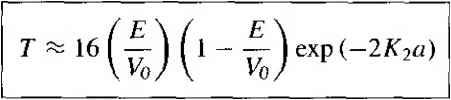

EXAMPLE 2.5

Objective

To ealeulate the probability of an electron tunneling through a potential barrier.

Consider an electron with an energy of 2 eV impinging on a potential barrier with Vo 20 eV anda widthof3 A.

Solution

Equation (2.62) is the tunneling probability. The factor К2 is

2m(Vo-E) /2(9.11 x 10- )(20 - 2)(1.6 x lO )

(1.054 X Ш-4)-

= 2.17 X 10* m

Then

T - 16(0-1)(] -0.1)exp[-2(2.17 x 10)(3 x lO )!

I-10

and finally

7 3.17 X 10

Comment

The tunneling probability may appear to be a small value, but the value is not zero. If a large number of particles impinge on a potential barrier, a significant number can penetrate the barrier.

E2.8

E2.9

TEST YOUR UNDERSTANDING

Estimate the tunneling probability of an electron tunneling through a rectangular barrier with a barrier height of Vy = 1 eV and a barrier width of 15 A. The electron energy is 0.20 eV. (Ol x 4LZ 1 suV)

For a rectangular potential barrier with a height of 2 cV and an electron with an energy of 0.25 eV, plot the tunneling probability versus barrier width over the range 2 5 Й < 20 A. Use a log scale for the tunneling probability. Е2Л0 A certain semiconductor device requires a tunneling probability of Г = 10 for an electron tunneling through a rectangular barrier with a barrier height of Vo = 0,4 eV, The eleclron energy is 0.04 eV. Determine the inaximum barrier width.

Additional applications of Schrodingers wave equation with various one-dimensional potential functions are found in problems at the end of the chapter. Several of these potential functions represent quantum well structures that are found in modern semiconductor devices.

*2.4 I EXTENSIONS OF THE WAVE THEORY TO ATOMS

So far in this chapter, we have considered several one-dimensional potential energy functions and solved Schrodingers time-independent wave equation to obtain the probability function of finding a particle at various positions. Consider now the one-electron, or hydrogen, atom potential function. We will only briefly consider the mathematical details and wave function solutions, but the results are extremely interesting and important.

2,4.1 The One-Electron Atom

The nucleus is a heavy, positively charged proton and the electron is a light, negatively charged particle that, in the classical Bohr theory, is revolving around the nucleus. The potential function is due to the coulomb attraction between the proton and electron and is given by

(2.63)

where is the magnitude of the electronic charge and 6o is the permittivity of free space. This potential function, although spherically symmetric, leads to a three-dimensional problem in spherical coordinates.

*Indicates sections that can be skipped without loss of continuity.

We may generalize the time-independent Schrodingers wave equation to three dimensions by writing

VV/( 0, Ф) + ~{Е - V(r))V(r, e, 0) - 0 (2.64)

where is the Laplacian operator and must be written in spherical coordinates for this case. The parameter mo is the rest mass of the electron.-* In spherical coordinates, Schrodingers wave equation may be written as

I д (

dr \ dr

, ~ (2.65)

The solution to Equation (2.65) can be determined by the separation-of-variables technique. We will assume that the solution to the time-independent wave equauon can be written in the form

ф(г, 0, Ф) = R(r) e() - Ф(0) (2.66)

where R,S, and Ф, are functions only of i9, and 0, respectively. Substituting this form of solution into Equation (2.65), we will obtain

sine Э / jdR\ 1 Э-Ф sine д /. эе\

----[r- H----- -h--- - ( sm (9--

R Br У Br J Ф Вф e BO \ BO J

(2.67)

We may note that the second term in Equation (2.67) is a function of ф only, while all the other terms are functions of either r or 6, We may then write that

1 9Ф

= -m (2.68)

Ф Вф-

where m is a separation of variables constant. The solution to Equation (2.68) is of the form

Ф - e (2.69)

Since the wave function must be single-valued, we impose the condition that m is an integer, or

/77 0, ±1, ±2, ±3,... (2.70)

The mass should be the rest mass of the two-particle system, but since the proton mass is much greater than the electron mass, the equivalent mass reduces to that of the electron.

Where m means the separation-of-variables constant developed historically. That meaning will be retained here even though there may be some confusion with the electron mass. In general, the mass parameter will be used in conjunction with a subscript.

Incorporating the separation-of-variables constant we can further separate the variables 9 and r and generate two additional separation-of-variables constants / and n. The separation-of-variables constants n,L and ш are known as quantum numbers and are related by

n = I, 2, 3,...

I - n - I, /7 - 2, 7 - 3,..., 0 m = /, / - I,..., 0

(2-71)

Each set of quantum numbers corresponds to a quantum state which the electron may occupy.

The electron energy may be written in the form

-moe

(2.72)

where n is the principal quantum number. The negative energy indicates that the electron is bound to the nucleus and we again see that the energy of the bound electron is quantized. If the energy were to become positive, then the electron would no longer be a bound particle and the total energy would no longer be quantized. Since the parameter n in Equation (2.72) is an integer, the total energy of the electron can take on only discrete values. The quantized energy is again a result of the particle being bound in a finite region of space.

TEST YOUR UNDERSTANDING

Е2Л1 Calculate the lowest energy (in electron volts) of an electron in a hydrogen atom. (Л3 9Т1- = 3 *W)

The solution of the wave equation may be designated by fnim where nj, and m are again the various quantum numbers. For the lowest energy state, n = 1Л = 0, and m = 0, and the wave function is given by

This function is spherically symmetric, and the parameter qq is given by

ao =-V = t).529 A

(2.73)

(2Л4)

and is equal to the Bohr radius.

The radial probability density function, or the probability of finding the electron at a particular distance from the nucleus, is proportional to the product i/f im and also to the differential volume of the shell around the nucleus. The probability