Time Base Generator

VERT. AMP. r1 i. CONTROL 1M >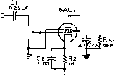

ntensity mod.

R15,47 К R 16.100

-O OUTPUT

R7,1S0K

Figure 2

TYPICAL AHflPLIFIER SCHEMATIC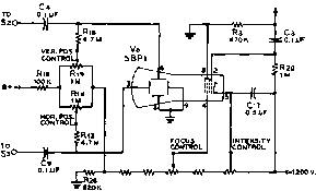

R2S R2 r23 R22

laoK leoK 0K 120K

R2t lOOK

the cathode-ray tube. Also, as shown in figure 1, S2 has been incorporated to by-pass the vertical amplifier and capacitively couple the input signal directly to the vertical deflection plate if so desired.

In figure 2, V, is a 6AC7 pentode tube which is used as the vertical amplifier. As the signal variations appear on the grid of V, variations in the plate current of will take place. Thus signal variations will appear in opposite phase and greatly amplified across the plate resistor, Rj. Capacitor Cj has been added a-cross Rj in the cathode circuit of Vj to flatten the frequency response of the amplifier at the high frequencies. This capacitor because of its low value has very little effect at low input frequencies, but operates more effectively as the frequency of the signal increases. The amplified signal delivered by Vj is now applied through the second half of switch Sj and capacitor C4 to the free vertical deflection plate of the cathode-ray tube (figure 3).

The Horizontol The circuit of the horizontal Amplifier amplifier and the circuit of

the vertical amplifier, described in the above paragrh, are similar. A switch in the input circuit makes provision for the input from the Horizontal Input terminals to be capacitively coupled to the grid of the horizontal amplifier or to the free horizontal deflection plate thus by-passing the amplifier, or for the output of the sweep generator to be capacitively coupled to the amplifier, as shown in figure 1.

The Time Base Investigation of electrical Generator wave forms by the use of a

cathode-ray tube frequently requires that some means be readily available to determine the variation in these wave forms with respect to time. When such a time base

is required, the patterns presented on the cathode-ray tube screen show the variation in amplitude of the input signal with respect to

Figure 3

SCHEMATIC OF CATHODE-RAY TUBE CIRCUITS

A 5BPIA caihoderay tube is used in this instrument. As shown, the necessary potentials for operating this tube are obtained from a voltage divider made up of resistors

f21 through R26 inc/usiVe. The intensity of the beam is adjusted by moving the corrfoct on R21- This adjusts the potential on the cathode more or less negative with respect to the grid which is operated at the full negative voltage~1200 volts. Focusing to the desired sharpness is accomplished by adjusting the contact on Rjj to provide the correct poterttial for anode no. I. Interde-pendency between the focus and the, intensity controls is inherent in all electrostatically focused cathode-ray tubes. In short, there Is an optimum setting of the focus control for every setting of the intensity control. The second alюde of the SBP1A is operated at ground poterttial in this Instrument. Also one of each pair of deflection plates is

operated at ground potential. The cathode is operated at a high negative potential (approximately 12(Ю volts) so that the total overall accelerating voltage of this tube is regarded as 1200 volts since the second artode is operated at ground poterttial. The vertical and horizontal positioning controls which are connected to their respective deflection plates are capable of supplying either a positive or negative d-c potential to the deflection plates. This permits the spot to be positioned at any desired place on the entire screen.

time. Such an arrangement is made possible by the inclusion in the oscilloscope of a Time Base-Generator. Th6 function of this generator is to move the spot across the screen at a constant rate from left to right between two selected points, to return the spot almost instantaneously to its original position, and to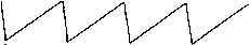

Figure 4 SAWTOOTH WAVE FORM

repeat this procedure at a specified rate. This action is accomplished by the voltage output from the time base (sweep) generator. The rate at which this voltage repeats the cycle of sweeping the spot across the screen is referred to as the sweep frequency. The sweep voltage necessary to produce the motion described above must be of a sawtooth waveform, such as that shown in figure 4.

The sweep occurs as the voltage varies from A to B, and the return trace as the voltage varies from В to C. If A-B is a straight line, the sweep generated by this voltage will be linear. It should be realized that the sawtooth sweep signal is only used to plot variations in the vertical axis signal with respect to time. Specialized studies have made necessary the use of sweep signals of various shapes which are introduced from an external source through the Horizontal Input terminals.

The Sowtooth The sawtooth voltage neces-Generator sary to obtain the linear time

base is generated by the circuit of figure 5, which operates as follows: A type 884 gas triode (V,) is used for the sweep generator tube. This tube contains an inert gas which ionizes when the voltage between the cathode and the plate reaches a certain value. The ionizing voltage depends upon the bias voltage of the tube, which is determined by the voltage divider resistors Ri2-Ri7-With a specific negative bias applied to the

884 tube, the tube will ionize (or fire) at a specific plate voltage.

Capacitors C10-c14 are selectively connected in parallel with the 884 tube. Resistor Rn limits the peak current drain of the gas triode. The plate voltage on this tube is obtained through resistors Rjg, R and R. The voltage applied to the plate of the 884 tube cannot reach the power supply voltage because of the charging effect this voltage has upon the capacitor which is connected across the tube. This capacitor charges until the plate voltage becomes high enough to ionize the gas in the tube. At this time, the 884 tube starts to conduct and the capacitor discharges through the tube until its voltage falls to the extinction potential of the tube. When the tube stops conducting, the capacitor voltage builds up until the tube fires again. As this action continues, it results in the sawtooth wave form of figure 4 appearing at the junction of Rj and Rj,.

Synchronization Provision has been made so the sweep generator may be synchronized from the vertical amplifier or from an external source. The switch S, shown in figure 5 is mounted on the front panel to be easily accessible to the operator.

If no synchronizing voltage is applied, the discharge tube will begin to conduct when the plate potential reaches the value of Ef (Firing Potential). When this breakdown takes place and the tube begins to conduct, the capacitor is discharged rapidly through the tube, and the plate voltage decreases until it reaches the extinction potential E. At this point conduction ceases, and the plate potential rises slowly as the capacitor begins to charge through R27 and Rjg. The plate potential will again reach a point of conduction and the circuit will start a new cycle. The rapidity of the plate voltage rise is dependent upon the circuit constants Rj Rj and the capacitor selected.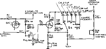

Figure 5

SCHEMATIC OF SWEEP GENERATOR

HANDBOOK

The Oscilloscope 173

Eb±

Ep vs £g

static control

f characteristic

Ep +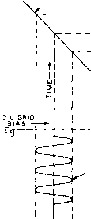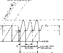

firing potential (d.c. bias)

firing I free run- potentia ning period with sync.

sjgnal

5vnc. signal applied to grid

Figure 6

ANALYSIS OF SYNCHRONIZATION OF TIME-BASE GENERATOR

C10-C14, as well as the supply voltage Ef The exact relationship is given by:

Where Ep=Capacitor voltage at time t

Eb=Supply voltage (B+ supply - cathode bias)

Ep=Firing potential or potential at which

time-base gas triode fires Ejj==Extinction potential or potential at which time-base gas triode ceases to conduct e=Base of natural logarithms t= Time in seconds

r=Resistance in ohms (Rj, + Rjj) c=Capacity in farads (C

105 iij 12j 135

or 14)

The frequency of oscillation will be approximately:

E,-E,

Under this condition (no synchronizing signal applied) the oscillator is said to be /гее running.

When a positive synchronizing voltage is applied to the grid, the firing potential of the tube is reduced. The tube therefore ionizes at a lower plate potential than when no grid signal is applied. Thus the applied snychroniz-ing voltage fires the gas-filled triode each

time the plate potential rises to a sufficient value, so that the sweep recurs at the same or an integral sub-multiple of the synchronizing signal rate. This is illustrated in figure 6.

Power Supply Figure 7 shows the power supply to be made up of two definite sections: a low voltage positive supply which provides power for operating the amplifiers, the sweep generator, and the positioning circuits of the cathode-ray tube; and the high voltage negative supply which provides the potentials necessary for operating the various

~i200v. i80k

Гг©

О

- о

3ISV. о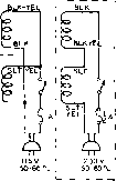

I 3LT

Figure 7

SCHEMATIC OF POWER SUPPLY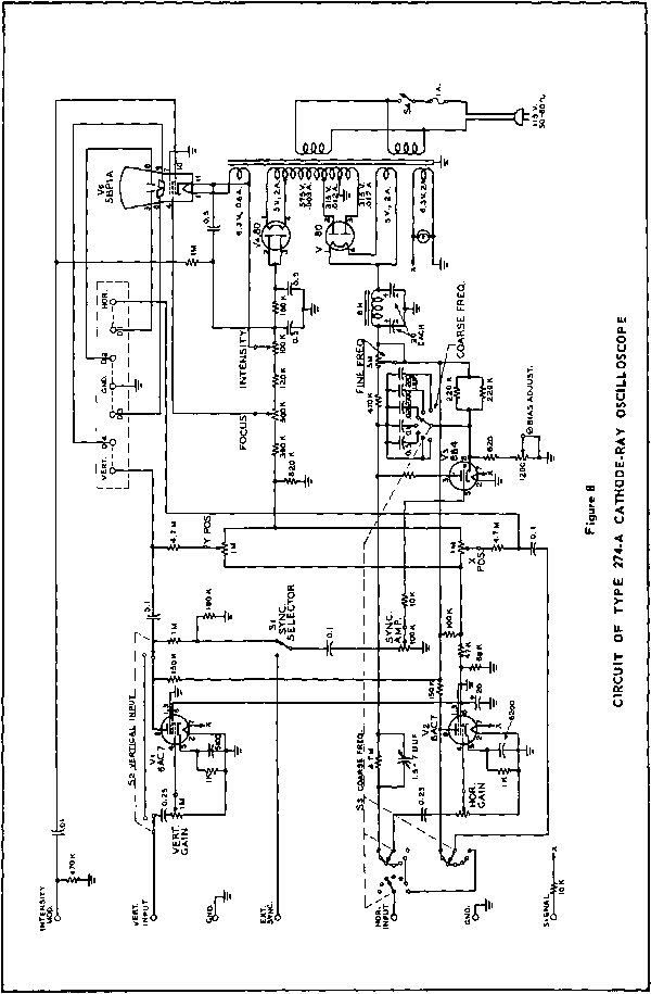

HANDBOOK

Display of Waveforms 175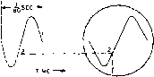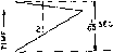

Figure 9

PROJECTION DRAWING OF A SINEWAVE APPLIED TO THE VERTICAL AXIS AND A SAWTOOTH WAVE OF THE SAME FREQUENCY APPLIED SIMULTANEOUSLY ON THE HORIZONTAL AXIS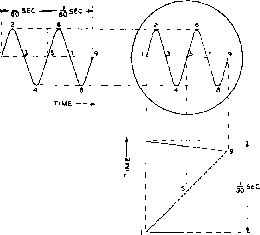

Figure 10

PROJECTION DRAWING SHOWING THE RESULTANT PATTERN WHEN THE FRE-QUENCYOF THE SAWTOOTH IS ONE-HALF OF THAT EMPLOYED IN FIGURE 9

electrodes of the cathode-ray tube, and for certain positioning controls.

The positive low voltage supply consists of full-wave rectifier (V5), the оифи! of which is filtered by a capacitor input filter (20-20 /zfd. and 8 H). It furnishes approximately 400 volts. The high voltage power supply employs a half wave rectifier tube, V4. The output of this rectifier is filtered by a resistance-capacitor filter consisting of 0.5-0.5 [ifd. and .18 M. A voltage divider network attached from the output of this filter obtains the proper operating potentials for the various electrodes of the cathode-ray tube. The complete schematic of the Du Mont 274-A Oscilloscope is shown in figure 8.

Display of Woveforms

Together with a working knowledge of the controls of the oscilloscope, an understanding of how the patterns are traced on the screen must be obtained for a thorough knowledge of oscilloscope operation. With this in mind a careful analysis of two fundamental waveform patterns is discussed under the following headings:

a. Patterns plotted against time (using the sweep generator for horizontal deflection).

b. Lissajous Figures (using a sine wave for horizontal deflection).

Patterns Plotted Against Time

A sine wave is typical of such a pattern and is convenient for this study. This

wave is amplified by the vertical amplifier and impressed on the vertical (Y-axis) deflection plates of the cathode-ray tube. Simultaneously the sawtooth wave from the time base generator is amplified and impressed on the horizontal (X-axis) deflection plates.

The electron beam moves in accordance with the resultant of the sine and sawtooth signals. The effect is shown in figure 9 where the sine and sawtooth waves are graphically represented on time and voltage axes. Points on the two waves that occur simultaneously are numbered similarly. For example, point 2 on the sine wave and point 2 on the sawtooth wave occur at the same instant. Therefore the position of the beam at instant 2 is the resultant of the voltages on the horizontal and vertical deflection plates at instant 2. Referring to figure 9, by projecting lines from the two point 2 positions, the position of the electron beam at instant 2 can be located. If projections were drawn from every other instantaneous position of each wave to intersect on the circle representing the tube screen, the intersections of similarly timed projections would trace out a sine wave.

In summation, figure 9 illustrates the principles involved in producing a sine wave trace on the screen of a cathode-ray tube. Each intersection of similarly timed projections represents the position of the electron beam acting under the influence of the varying voltage waveforms on each pair of deflection plates. Figure 10 shows the effect on the pattern of decreasing the frequency of the sawtooth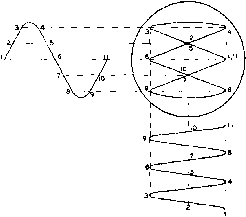

Figure 12

METHOD OF CALCULATING FREQUENCY RATIO OF LISSAJOUS FIGURES

Figure 11

PROJECTION DRAWING SHOWING THE RESULTANT LISSAJOUS PATTERN WHEN A SINE WAVE APPLIED TO THE HORIZONTAL AXIS IS THREE TIMES THAT AP-PLIED TO THE VERTICAL AXIS

wave. Any recurrent waveform plotted against time can be displayed and analyzed by the same procedure as used in these examples.

The sine wave problem just illustrated is typical of the method by which any waveform can be displayed on the screen of the cathode-ray tube. Such waveforms as square wave, sawtooth wave, and many more irregular recurrent waveforms can be observed by the same method explained in the preceding paragraphs.

Obtaining a Lissaious I. The horizontal am-Pottern on fhe screen plifier should be discon-Oseilloscope Settings nected from the sweep oscillator. The signal to be examined should be connected to the horizontal amplifier of the oscilloscope.

2. An audio oscillator signal should be connected to the vertical amplifier of the oscillo-scce.

3. By adjusting the frequency of the audio oscillator a stationary pattern should be obtained on the screen of the oscilloscope. It is not necessary to stop the pattern, but merely to slow it up enough to count the loops at the side of the pattern.

4. Count the number of loops which intersect an imaginary vertical line AB and the number of loops which intersect the imaginary horizontal line ВС as in figure 12. The ratio of the number of loops which intersect AB is to

Lissajous Figures

Another fundamental pattern is the Lissajous figure, named after the 19th century French scientist. This type of pattern is of particular use in determining the frequency ratio between two sine wave signals. If one of these signals is known, the other can be easily calculated from the pattern made by the two signals upon the screen of the cathode-ray tube. Common practice is to connect the known signal to the horizontal channel and the unknown signal to the vertical channel.

The presentation of Lissajous figures can be analyzed by the same method as previously used for sine wave presentation. A simple example is shown in figure 11. The frequency ratio of the signal on the horizontal axis to the signal on the vertical axis is 3 to 1. If the known signal on the horizontal axis is 60 cycles per second, the signal on the vertical axis is 20 cycles.

(j) RATIO hi

ratio гч

@ ratio 1.5

ratio 10; i

Figure 13 OTHER LISSAJOUS PATTERNS

HANDBOOK

Lissajous Figures 177

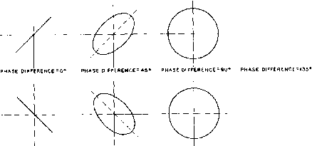
PHASE DIFFkRENCE ieO> PHASE Dl FFERENCE =225 PHASE DIFFERENCE 270- PHASE DIFFERENCE 3 I 5

Figure H

LISSAJOUS PATTERNS OBTAINED FROM THE MAJOR PHASE DIFFERENCE ANGLES

the number of loops which intersect ВС as the frequency of the horizontal signal is to the frequency of the vertical signal.

Figure 13 shows other examples of Lissajous figures. In each case the frequency ratio shown is the frequency ratio of the signal on the horizontal axis to that on the vertical axis.

Phase Differ- Coming under the heading of once Patterns Lissajous figures is the method used to determine the phase difference between signals of the same frequency. The patterns involved take on the form of ellipses with different degrees of eccentricity.

The following steps should be taken to obtain a phase-difference pattern:

1. With no signal input to the oscilloscope, the spot should be centered on the screen of the tube.

2. Connect one signal to the vertical amplifier of the oscilloscope, and the other signal to the horizontal amplifier.

3. Connect a common ground between the two frequencies under investigation and the oscilloscope.

4. Adjust the vertical amplifier gain so as to give about 3 inches of deflection on a 5 inch tube, and adjust the calibrated scale of the oscilloscope so that the vertical axis of the scale coincides precisely with the vertical deflection of the spot.

5. Remove the signal from the vertical amplifier, being careful not to change the setting of the vertical gain control.

6. Increase the gain of the horizontal amplifier to give a deflection exactly the same as that to which the vertical am-

plifier control is adjusted (3 inches). Reconnect the signal to the vertical amplifier.

The resulting pattern will give an accurate picture of the exact phase difference between the two waves. If these two patterns are exactly the same frequency but different in phase and maintain that difference, the pattern on the screen will remain stationary. If, however, one of these frequencies is drifting slightly, the pattern will drift slowly through 360 . The phase angles of 0°, 45°, 90°, 135°, 180°, 225°, 270°, 315° are shown in figure 14.

Each of the eight patterns in figure 14 can be analyzed separately by the previously used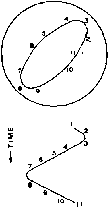

Figure 15

PROJECTION DRAWING SHOWING THE RESULTANT PHASE DIFFERENCE PATTERN OF TWO SINE WAVES 45° OUT OF PHASE

У INTERCEPT = .S-

Y MAXIMUM- I

У INTERCEPT= 7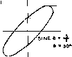

V MAXIMUM-1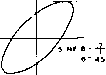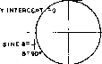

Y MAXIMUM- i y.

=1 YMAXIMUM

Y INTERCEPT.5

r INTERCEPT =.7

Figure 16

EXAMPLES SHOWING THE USE OF THE FORMULA FOR DETERMINATION OF PHASE

DIFFERENCE

projection method. Figure 15 shows two sine waves which differ in phase being projected on to the screen of the cathode-ray tube. These signals represent a phase difference of 45°. It is extremely important: (1) that the spot has been centered on the screen of the cathode-ray tube, (2) that both the horizontal and vertical amplifiers have been adjusted to give exactly the same gain, and (3) that the calibrated scale be originally set to coincide with the displacement of the signal along the vertical axis. If the amplifiers of the oscilloscope are not used for conveying the signal to the deflection plates of the cathode-ray tube, the coarse frequency switch should be set to hori-zontal input direct and the vertical input

switch to direct and the outputs of the two signals must be adjusted to result in exactly the same vertical deflection as horizontal deflection. Once this deflection has been set by either the oscillator output controls or the amplifier gain controls in the oscillograph, it should not be changed for the duration of the measurement.

Determination of the Phase Angle

The relation commonly used in determining the phase angle between signals is:

Sine в :

Y intercept

Y maximum

Figure 17

TRAPEZOIDAL MODULATION PATTERN

Figure 18

MODULATED CARRIER WAVE PATTERN

2A SA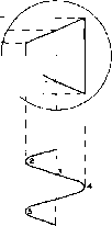

Figure 19

PROJECTION DRAWING SHOWING TRAPE-ZOIDAL PATTERN

HANDBOOK

Trapezoidal Pattern 179

MODULATED CARRIER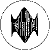

RF. POWER AMPLIFIER

Figure 20

PROJECTION DRAWING SHOWING MODULATED CARRfER WAVE PATTERN

where = phase angle between signals

Y intercept = point where ellipse crosses ver-

tical axis measured in tenths of inches. (Calibrations on the calibrated screen)

Y maximum = highest vertical point on ellipse

in tenths of inches

Several examples of the use of the formula are given in figure 16. In each case the Y intercept and Y maximum are indicated together with the sine of the angle and the angle itself. For the operator to observe these various patterns with a single signal source such as the test signal, there are many types of phase shifters which can be used. Circuits can be obtained from a number of radio text books. The procedure is to connect the original signal to the horizontal channel of the oscilloscope and the signal which has passed through the phase shifter to the vertical channel of the oscilloscope, and follow the procedure set forth in this discussion to observe the various phase shift patterns.

9-4 Monitoring Transmitter

Performance with the Oscilloscope

The oscilloscope may be used as an aid for the proper operation of a radiotelephone transmitter, and may be used as an indicator of the overall performance of the transmitter output signal, and as a modulation monitor.

Waveforms There are two types of patterns that can serve as indicators, the trapezoidal pattern (figure 17) and the modu-

MODULATOR STAGE

TO ANTENNA

, EACH 1M, 1W

-((--W-VW-<W-M-

SOOUUF 10000 V. -TV CAPACITOR

LC TUNES TO OP- , ERATING FREOueNCyJ,

NOTE /f я. f. pickup is insufficient, Л tuned circuit мау- be used at The oscilloscope as shown.

Figure 21

MONITORING CIRCUIT FOR TRAPEZOIDAL MODULATION PATTERN

lated wave pattern (figure 18). The trapezoidal pattern is presented on the screen by impressing a modulated carrier wave signal on the vertical deflection plates and the signal that modulates the carrier wave signal (the modulating signal) on the horizontal deflection plates. The trapezoidal pattern can be analyzed by the method used previously in analyzing waveforms. Figure 19 shows how the signals cause the electron beam to trace out the pattern.

The modulated wave pattern is accomplished by presenting a modulated carrier wave on the vertical deflection plates and by using the time-base generator for horizontal deflection. The modulated wave pattern also can be used for analyzing waveforms. Figure 20 shows how the two signals cause the electron beam to trace out the pattern.

The Trapezoidal Pattern

The oscilloscope connections for obtaining a trapezoidal pattern are shown in figure 21. A portion of the audio output of the transmitter modulator is applied to the horizontal input of the oscilloscope. The vertical amplifier of the oscilloscope is disconnected, and a small amount of modulated r-f energy is coupled directly to the vertical deflection

plates of the oscilloscope. A small pickup

loop, loosely coupled to the final amplifier tank circuit and connected to the vertical de-

E MAX

TRAPEZOIDAL WAVE PATTERN Figure 22 Figure 23

(LESS THAN 100% MODULATION) (100% MODULATION)

Figure 24 (OVER MODULATION)

flection plates by a short length of coaxial line will suffice. The amount of excitation to the plates of the oscilloscope may be adjusted to provide a pattern of convenient size. Upon modulation of the transmitter, the trapezoidal pattern will appear. By changing the degree of modulation of the carrier wave the shape of the pattern will change. Figures 22 and 23 show the trapezoidal pattern for various degrees of modulation. The percentage of modulation may be determined by the following formula:

Modulation percentage

+ E,

X 100

where £ ,3 and Ej are defined as in figure 22.

An overmodulated signal is shown in figure

The Moduioted Wave Pattern

The oscilloscope connections for obtaining a modulated wave pattern are shown in

R F. POWER AMPLIFIER

TO ANTENNA

USE INTERNAL

SWEEP. .0,.

at FROM MODULATOR

LC TUNES TO OPERATING FREOUENCY

Figure 25

MONITORING CIRCUIT FOR MODULATED WAVE PATTERN

figure 25. The internal sweep circuit of the oscilloscope is applied to the horizontal plates, and the modulated r-f signal is applied to the vertical plates, as described before. If desired, the internal sweep circuit may be sny-chronized with the modulating signal of the transmitter by applying a small portion of the modulator оифи! signal to the external sync post of the oscilloscope. The percentage of modulation may be determined in the same fashion as with a trapezoidal pattern. Figures 26, 27 and 28 show the modulated wave pattern for various degrees of modulation.

9-5 Receiver I-F Alignment

with an Oscilloscope

The alignment of the i-f amplifiers of a receiver consists of adjusting all the tuned circuits to resonance at the intermediate frequency and at the same time to permit passage of a predetermined number of side bands. The best indication of this adjustment is a resonance curve representing the response of the i-f circuit to its particular range of frequencies.

As a rule medium and low-priced receivers use i-f transformers whose bandwidth is about 5 kc. on each side of the fundamental frequency. The response curve of rhese i-f transformers is shown in figure 29- High fidelity receivers usually contain i-f transformers which have a broader bandwidth which is usually 10 kc. on each side of the fundamental. The response curve for this type transformer is shown in figure 30.

Resonance curves such as these can be displayed on the screen of an oscilloscope. For a complete understanding of the procedure it is important to know how the resonance curve is traced.