 |
 |
 |
| Главная Журналы Популярное Audi - почему их так назвали? Как появилась марка Bmw? Откуда появился Lexus? Достижения и устремления Mercedes-Benz Первые модели Chevrolet Электромобиль Nissan Leaf |
Главная » Журналы » Simple coaxial reflectometer 1 2 3 4 5 6 7 8 ... 80 HANDBOOK Vector Algebra 51 VOLTAGE DROP ACROSS  drop across resistor - 70.a /45 VliNE voltage = 1001, drop across xc = 106.2/~ net drop across Xl+ Хс = 70,8Ад5 Figure 14 Graphical construction of tho voltage drops associated with the series R-L-C circuit of figure 13, El =35.4135° = 35.4 (cos 135°+ j sin 135°) = 35.4 (-0.707 + jO.707) = -25 + j25 Ec = 106.2 45° = 106.2 (cos-45°+ j sin-45°) = 106.2 (0.707 -jO.707) = 75 -)75 Er + El + f с = (50 + )50) + (-25 + j25) + (75-j75) = (50-25 + 75)+ j (50 + 25-75) = 100 + jO = 100 /-0°, which is equal to the supply voltage. Checking by It is frequently desirable Construction on the to check computations in-Complex Plane volving complex quantities by constructing vectors representing the quantities on the complex plane. Figure 14 shows such a construction for the quantities of the problem just completed. Note that the answer to the problem may be checked by constructing a parallelogram with the voltage drop across the resistor as one side and the net voltage drop across the capacitor plus the inductor (these may be added algrebraically as they are 180° out of phase) as the adjacent side. The vector sum of these two voltages, jirhich is represented by the diagonal of the parallelogram, is equal to the supply voltage of 100 volts at zero phase angle. Resistance and Re- Qctonee in Parallel In a series circuit, such as just discussed, the current through all the ele-  parallel CIRCUIT equivalent series CIRCUIT Figure 15 THE EQUIVALENT SERIES CIRCUIT Showing a parallel R-C circuit and the equivalent series R-C circuit which represents the same net Impedance as the parallel circuit. ments which go to make up the series circuit is the same. But the voltage drops across each of the components are, in general, different from one another. Conversely, in a parallel RLC or RX circuit the voltage is, obviously, the same across each of the elements. But the currents through each of the elements are usually different. There are many ways of solving a problem involving paralleled resistance and reactance; several of these ways will be described. In general, it may be said that the impedance of a number of elements in parallel is solved using the same relations as are used for solving resistors in parallel, except that complex quantities are employed. The basic relation is: 1 1 -+ - + Ztot Z, Zj Zj or when only two impedances are involved: Ztot- Zi + Zj As an example, using the two-impedance relation, take the simple case, illustrated in figure 15, of a resistance of 6 ohms in parallel with a capacitive reactance of 4 ohms. To simplify the first step in the computation it is best to put the impedances in the polar form for the numerator, since multiplication is involved, and in the rectangular form for the addition in the denominator. Ztot (6 0°) (4 1.-90°) 6-j4 24 1-90° 6-j4 Then the denominator is changed to the polar form for the division operation: в = tan- - = tan- - 0.667 = - 33-7° 6 Izl = Then: Ztot COS - 33.7° 0.832 6 -j4 = 7.21 L-ЪЪ.Т - 7.21 ohms 24 A-90° ;=3.33 A-56.3° 7.21 /.-33.7° 3-33 ( cos - 56.3° + i sin -56.3°) 3.33 [0.5548 +j (-0.832)] 1.85 - j 2.77 ::r2 Ег E2-E1 Ri + Rz El - =т^сг Ег = XCi +XC2 E2 = Ei  © ® © Figure 16 SIMPLE AC VOLTAGE DIVIDERS EquivalenI Series Through the series of op-Circuit erations in the previous paragraph we have converted a circuit composed of two impedances in parallel into an equivalent series circuit composed of impedances in series. An equivalent series circuit is one which, as far as the terminals are concerned, acts identically to the original parallel circuit; the current through the circuit and the power dissipation of the resistive elements are the same for a given voltage at the specified frequency. We can check the equivalent scries circuit of figure 15 with respect to the original circuit by assuming that one volt a.c. (at the frequency where the capacitive reactance in the parallel circuit is 4 ohms) is applied to the terminals of both. In the parallel circuit the current through the resistor will be % ampere (0. l66a.) while the current through the capacitor will be j V4 ampere ( + j 0.25 a.). The total current will be the sum of these two currents, or O.I66 + j 0.25 a. Adding these vectorially we obtain: in = V0.166 + 0.25 = VO.O9 =0.3 a. The dissipation in the resistor will be l/6 = 0.166 watts. In the case of the equivalent series circuit the current will be: , , E 1 1 =-=--0.3 a. \z\ 3.33 And the dissipation in the resistor will be: W = lR = 0.3x 1.85 = 0.9 x 1.85 = 0.166 watts So we see that the equivalent series circuit checks exactly with the original parallel circuit. Parallel RLC In solving a more complicated Circuits circuit made up of more than two impedances in parallel we may elect to use either of two methods of solution. These methods are called the admittance method and the assumed-voltage method. However, the two methods are equivalent sinceboth use the sum-of-reciprocals equation: 1111 =- +- +-..... Zfgt Zl Zj In the admittance method we use the relation Y = l/Z, where Y = G-b jB; Y is called the admittance, defined above, G is the conductance or R/Z and В is the susceptance or -X/Z. Then Ytot = 1/Ztot = Yi + Yj + Y3---- In the assumed-voltage method we multiply both sides of the equation above by E, the assumed voltage, and add the currents, as: E E E Е III tOt 1 2 3 Then the impedance of the parallel combination may be determined from the relation: Ztot = E/Iz tot AC Voltage Voltage dividers for use with Dividers alternating current are quite similar to d-c voltage dividers. However, since capacitors and inductors oppose the flow of a-c current as well as resistors, voltage dividers for alternating voltages may take any of the configurations shown in figure 16. Since the impedances within each divider are of the same type, the output voltage is in phase with the input voltage. By using combinations of different types of impedances, the phase angle of the output may be shifted in relation to the input phase angle at the same time the amplitude is reduced. Several dividers of this type are shown in figure 17, Note that the ratio of output voltage to input voltage is equal to the ratio of the output impedance to the total divider impedance. This relationship is true only if negligible current is drawn by a load on the ouфut terminals.   xl-xc © Ea = Ei Ун+ (xl-xc)2 XL e4 = Et Vrh+(xl-xc)h xl-xc 1r2 + (xl-xc)2 Figure 17 COMPLEX A-C VOLTAGE DIVIDERS Resonant Circuits A series circuit such as shown in figure 18 is said to be in resonance when the applied frequency is such that the capacitive reactance is exactly balanced by the inductive reactance. At this frequency the two reactances will cancel in their effects, and the impedance of the circuit will be at a minimum so that maximum current will flow. In fact, as shown in figure 19 the net impedance of a series circuit at resonance is equal to the resistance which remains in the circuit after the reactances have been cancelled. Resonant Frequency Some resistance is always present in a circuit because it is possessed in some degree by both the inductor and the capacitor. If the frequency of the alternator E is varied from nearly zero to some high frequency, there will be one particular frequency at which the inductive reactance and capacitive reactance will be equal. This is known as the resonant frequency, and in a series circuit it is the frequency at which the circuit current will be a maximum. Such series resonant circuits are chiefly used when it is desirable to allow a certain frequency to pass through the circuit (low impedance to this frequency), while at the same time the circuit is made to offer considerable opposition to currents of other frequencies. Figure 18 SERIES RESONANT CIRCUIT If the values of inductance and capacitance both are fixed, there will be only one resonant frequency. If both the inductance and capacitance are made variable, the circuit may then be changed or tuned, so that a number of combinations of inductance and capacitance can resonate at the same frequency. This can be more easily understood when one considers that inductive reactance and capacitive reactance travel in opposite directions as the frequency is changed. For example, if the frequency were to remain constant and the values of inductance and capacitance were then changed, the following combinations would have equal reactance: Frequency is constant at 60 cycles. L is expressed in henrys. С is expressed in microfarads (.000001 farad.) L Xl С Xc .265 100 26.5 100 2.65 1,000 2.65 1,000 26.5 10,000 .265 10,000 265-00 100,000 .0265 100,000 2,650.00 1,000,000 .00265 1,000,000 Frequency From the formula for reson-of Resonance ance, 2fffL = l/2!7fC, the resonant frequency is determined: 2n-VLC where f = frequency in cycles, L = inductance in henrys, С = capacitance in farads. It is more convenient to express L and С in smaller units, especially in making radio-frequency calculations; f can also be expressed in megacycles or kilocycles. A very useful group of such formulas is: 25,330 , 25,330 f =- or L =--or С 25,330 fL where f = frequency in megacycles, L = inductance in microhenrys, С = capacitance in micromicrofarads.  Figure 19 IMPEDANCE OF A SERIES-RESONANT CIRCUIT Showing fhe vorfatfon (n reoclonce of rhe separata elements and In fhe net Impedance of о series resonant circuit (such as figure 18) with changing frequency. The vertical line Is drawn at the point of resonance fX - Xj. = 0) in the series circuit. Impedance of Series The impedance across Resonant Circuits the terminals of a series resonant circuit (figure 18) is: where Z = impedance in ohms, r = resistance in ohms, Xc = capacitive reactance in ohms, Xl = inductive reactance in ohms. From this equation, it can be seen that the impedance is equal to the vector sum of the circuit resistance and the difference between the two reactances. Since at the resonant frequency Xl equals X, the difference between them (figure 19) is zero, so that at resonance the impedance is simply equal to the resistance of the circuit; therefore, because the resistance of most normal radio-frequency circuits is of a very low order, the impedance is also low. At frequencies higher and lower than the resonant frequency, the difference between the reactances will be a definite quantity and will add with the resistance to make the impedance higher and higher as the circuit is tuned off the resonant frequency. If Xc should be greater than Xl, then the term (Xl - Xc) will give a negative number. However, when the difference is squared the product is always positive. This means that the smaller reactance is subtracted from the larger, regardless of whether it be capacitive or inductive, and the difference squared. (J -I I О I- z z < UJ Q (1 IL
FREQUENCY Figure 20 RESONANCE CURVE Shewing the increase in Impedance at resonance for a parallel-resonant circuit, and similarly, the Increase In current at resonance for a series-resonant circuit. The sharpness of resonance is determined by the 0 of the circuit, as Illustrated by a comparison between A, B. and C. Current and Voltage in Series Resonant Circuits Ohms law. Formulas for calculating currents and voltages in a series resonant circuit are similar to those of I=- E = 1Z Z The complete equations: Vr%(XL-Xc) E =1 Vt - Xc) Inspection of the above formulas will show the following to apply to series resonant circuits: When the impedance is low, the current will be high; conversely, when the impedance is high, the current will be low. Since it is known that the impedance will be very low at the resonant frequency, it follows that the current will be a maximum at this point. If a graph is plotted of the current against the frequency either side of resonance, the resultant curve becomes what is known as a resonance curve. Such a curve is shown in figure 20, the frequency being plotted against current in the series resonant circuit. Several factors will have an effect on the shape of this resonance curve, of which re- HANDBOOK Circuit Q 55 sistance and L-to-C ratio are the important considerations. The curves В and С in figure 20 show the effect of adding increasing values of resistance to the circuit. It will be seen that the peaks become less and less prominent as the resistance is increased; thus, it can be said that the selectivity of the circuit is thereby decreased. Selectivity in this case can be defined as the ability of a circuit to discriminate against frequencies adjacent to the resonant frequency, Volfage Across Coil Because the a.c. or r-f and Capacitor in voltage across a coil and Series Circuit capacitor is proportional to the reactance (for a given current), the actual voltages across the coil and across the capacitor may be many times greater than the terminal voltage of the circuit. At resonance, the voltage across the coil (or the capacitor) is Q times the applied voltage. Since the Q (or merit factor) of a series circuit can be in the neighborhood of 100 or more, the voltage across the capacitor, for example, may be high enough to cause flashover, even though the applied voltage is of a value considerably below that at which the capacitor is rated. Circuit Q - Sharp- An extremely important ness of Resonance property of a capacitor or an inductor is its factor-of-merit, more generally called its Q. It is this factor, Q, which primarily determines the sharpness of resonance of a tuned circuit. This factor can be expressed as the ratio of the reactance to the resistance, as follows: 27rfL where R = total resistance. Skin Effect The actual resistance in a wire or an inductor can be far greater than the d-c value when the coil is used in a radio-frequency circuit; this is because the current does not travel through the entire cross-section of the conductor, but has a tendency to travel closer and closer to the surface of the wire as the frequency is increased. This is known as the skin effect. The actual current-carrying portion of the wire is decreased, as a result of the skin effect, so that the ratio of a-c to d-c resistance of the wire, called the resistance ratio, is increased. The resistance ratio of wires to be used at frequencies below about 500 kc. may be materially reduced through the use of litz wire. Litz wire, of the type commonly used to wind the coils of 455*kc. i-f transformers, may consist of 3 to 10 strands of insulated wire, about No. 40 in size, with the individual strands connected together only at the ends of the coils. Variation of Q Examination of the equation with Frequency for determining Q might give rise to the thought that even though the resistance of an inductor increases with frequency, the inductive reactance does likewise, so that the Q might be a constant. Actually, however, it works out in practice that the Q of an inductor will reach a relatively broad maximum at some particular frequency. Hence, coils normally are designed in such a manner that the peak in their curve of Q with frequency will occur at the normal operating frequency of the coil in the circuit for which it is designed. The Q of a capacitor ordinarily is much higher than that of the best coil. Therefore, it usually is the merit of the coil that limits the overall Q of the circuit. At audio frequencies the core losses in an iron-core inductor greatly reduce the Q from the value that would be obtained simply by dividing the reactance by the resistance. Obviously the core losses also represent circuit resistance, just as though the loss occurred in the wire itself. Parallel In radio circuits, parallel reson-Resononce ance (more correctly termed anti-resonance) is more frequently encountered than series resonance; in fact, it is the basic foundation of receiver and transmitter circuit operation. A circuit is shown in figure 21. The Tonk In this circuit, as contrasted with Circuit a circuit for series resonance, L (inductance) and С (capacitance) are connected in parallel, yet the combination can be considered to be in series with the remainder of the circuit. This combination of L and C, in conjunction with R, the resistance which is principally included in L, is sometimes called a tank circuit because it effectively functions as a storage tank when incorporated in vacuum tube circuits. Contrasted with series resonance, there are two kinds of current which must be considered in a parallel resonant circuit: (1) the line current, as read on the indicating meter Mi, (2) the circulating current which flows within the parallel L-C-R portion of the circuit. See figure 21. At the resonant frequency, the line current (as read on the meter M,) will drop to a very low value although the circulating current in the L-C circuit may be quite large. It is interesting to note that the parallel resonant circuit acts in a distinctly opposite manner to that of a series resonant circuit, in which the  о L О -WWW- Figure 21 PARALLEL-RESONANT CIRCUIT The inductance l and eapecitanct с comprise the reactive elements of the parallel-resonant (anti-resonant) tank circuit, and the resistance R indicates the sum of the r-f resistance of the coll and capacitor, plus the resistance coupled into the circuit from the external load. In most cases the tuning capacitor has much lower r-f resistance than the call and con therefore be ignored in comparison with the call resistance and the coupied-ln resistance. The instrument Ml indicates the line current which keeps the circuit in a state of oscillation - this current Is the same os the fundamental component of the plate current of a Class С amplifier which might be feeding the tank circuit. The instrument Ui Indicates the tank current which is equal to the line current multiplied by the operating 0 of the tank circuit. current is at a maximum and the impedance is minimum at resonance. It is for this reason that in a parallel resonant circuit the principal consideration is one of impedance rather than current. It is also significant that the impedance curve for parallel circuits is very nearly identical to that of the current curve for series resonance. The impedance at resonance is expressed as: (27rfL) where Z = impedance in ohms, L = inductance in henrys, f = frequency in cycles, R = resistance in ohms. Or, impedance can be expressed as a function of Q as: Z = ZfffLQ, showing tht the impedance of a circuit is directly proportional to its effective Q at resonance. The curves illustrated in figure 20 can be applied to parallel resonance. Reference to the curve will show that the effect of adding resistance to the circuit will result in both a broadening out and lowering of the peak of the curve. Since the voltage of the circuit is directly proportional to the impedance, and since it is this voltage that is applied to the grid of the vacuum tube in a detector or am- plifier circuit, the impedance curve must have a sharp peak in order for the circuit to be selective. If the curve is broad-topped in shape, both the desired signal and the interfering signals at close proximity to resonance will give nearly equal voltages on the grid of the tube, and the circuit will then be nonselective; i.e., it will tune broadly. Effect of L/C Ratio In order that the highest in Parallel Circuits possible voltage can be developed across a parallel resonant circuit, the impedance of this circuit must be very high. The impedance will be greater with conventional coils of limited Q when the ratio of inductance-to-capacitance is great, that is, when L is large as compared with C. When the resistance of the circuit is very low, Xl will equal X at maximum impedance. There are innumerable ratios of L and С that will have equal reactance, at a given resonant frequency, exactly as in the case in a series resonant circuit. In practice, where a certain value of inductance is tuned by a variable capacitance over a fairly wide range in frequency, the L/C ratio will be small at the lowest frequency endandlarge atthe high-frequency end. The circuit, therefore, will have unequal gain and selectivity at the two ends of the band of frequencies which is being tuned. Increasing the Q of the circuit (lowering the resistance) will obviously increase both the selectivity and gain. Circulating Tank The Q of a circuit has Current at Resonance a definite bearing on the circulating tank current at resonance. This tank current is very nearly the value of the line current multiplied by the effective circuit Q. For example: an r-f line current of 0.050 amperes, with a circuit Q of 100, will give a circulating tank current of approximately 5 amperes. From this it can be seen that both the inductor and the connecting wires in a circuit with a high Q must be of very low resistance, particularly in the case of high power transmitters, if heat losses are to be held to a minimum. Because the voltage across the tank at resonance is determined by the Q, it is possible to develop very high peak voltages across a high Q tank with but little line current. Effect of Coupling on Impedance output circuit, the Q of the parallel coupling becomes (tighter) coupling If a parallel resonant circuit is coupled to another circuit, such as an antenna impedance and the effective circuit is decreased as the closer. The effect of closer is the same as though an   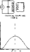 OVERCOUPLING LOW q  © ® ® Figure 22 EFFECT OF COUPLING ON CIRCUIT IMPEDANCE AND Q actual resistance were added in series with the parallel tank circuit. The resistance thus coupled into the tank circuit can be considered as being reflected from the output or load circuit to the driver circuit. The behavior of coupled circuits depends largely upon the amount of coupling, as shown in figure 22. The coupled current in the secondary circuit is small, varying with frequency, being maximum at the resonant frequency of the circuit. As the coupling is increased between the two circuits, the secondary resonance curve becomes broader and the resonant amplitude increases, until the reflected resistance is equal to the primary resistance. This point is called the critical coupling point. With greater coupling, the secondary resonance curve becomes broader and develops double resonance humps, which become more pronounced and farther apart in frequency as the coupling between the two circuits is increased. Tank Circuit When the plate circuit of a Flywheel Effect Class В or Class С operated tube is connected to a parallel resonant circuit tuned to the same frequency as the exciting voltage for the amplifier, the plate current serves to maintain this L/C circuit in a state of oscillation. The plate currentis supplied in short pulses which do not begin to resemble a sine wave, even though the grid may be excited by a sine-wave voltage. These spurts of plate current are converted into a sine wave in the plate tank circuit by virtue of the Q or flywheel effect of the tank. If a tank did not have some resistance losses, it would, when given a kick with a single pulse, continue to oscillate indefinitely. With a moderate amount of resistance or friction in the circuit the tank will still have inertia, and continue to oscillate with decreasing amplitude for a time after being given a kick. With such a circuit, almost pure sine-wave voltage will be developed across the tank circuit even though power is supplied to the tank in short pulses or spurts, so long as the spurts are evenly spaced with respect to time and have a frequency that is the same as the resonant frequency of the tank. Another way to visualize the action of the tank is to recall that a resonant tank with moderate Q will discriminate strongly against harmonics of the resonant frequency. The distorted plate current pulse in a Class С amplifier contains not only the fundamental frequency (that of the grid excitation voltage) but also higher harmonics. As the tank offers low impedance to the harmonics and high impedance to the fundamental (being resonant to the latter), only the fundamental - a sine-wave voltage - appears across the tank circuit in substantial magnitude. Loaded and Confusion sometimes exists as Unloaded Q to the relationship between the unloaded and the loaded Q of the tank circuit in the plate of an r-f power amplifier. In the normal case the loaded Q of the tank circuit is determined by such factors as the operating conditions of the amplifier, bandwidth of the signal to be emitted, permissible level of harmonic radiation, and such factors. The normal value of loaded Q for an r-f amplifier used for communications service is from perhaps 6 to 20. The unloaded Q of the tank circuit determines the efficiency of the output circuit and is determined by the losses in the tank coil, its leads and plugs and jacks if any, and by the losses in the tank capacitor which ordinarily are very low. The unloaded Q of a good quality large diameter tank coil in the high-frequency range may be as high as 500 to 800, and values greater than 300 are quite common. Tank Circuit Since the unloaded Q of a tank Efficiency circuit is determined by the minimum losses in the tank, vAiile the loaded Q is determined by useful loading of the tank circuit from the external load in addition to the internal losses in the tank circuit, the relationship between the two Q values determines the operating efficiency of the tank circuit. Expressed in the form of an equation, the loaded efficiency of a tank circuit is: Tank efficiency = 1 X 100 where Qu = unloaded Q of the tank circuit Qi = loaded Q of the tank circuit As an example, if the unloaded Q of the tank circuit for a class С r-f power amplifier is 400, and the external load is coupled to the tank circuit by an amount such that the loaded Q is 20, the tank circuit efficiency will be: eff. = (1 - 20/400) X 100, or (1 - 0.05) x 100, or 95 per cent. Hence 5 per cent of the power output of the Class С amplifier will be lost as heat in the tank circuit and the remaining 95 per cent will be delivered to the load. FUNDAMENTAL SINE WAVe(A) FUNDAMENTAL PLUS 3RD HARMONICQ J 3RD HARMONIC  Figure 23 COMPOSITE WAVE-FUNDAMENTAL PLUS THIRD HARMONIC  FUNDAMENTAL PLUS 3R0 HARMONIC FUNDAMENTAL PLUS 3RD ANO 5TH HARMONICsjgJ -STH HARMONIC (D)  Figure 24 THIRD HARMONIC WAVE PLUS FIFTH HARMONIC 3-3 Nonsinusoidal Vfaves and Transients Pure sine waves, discussed previously, are basic wave shapes. Waves of many different and complex shape are used in electronics, particularly square waves, saw-tooth waves, and peaked waves. Wove Composition Any periodic wave (one that repeats itself in definite time intervals) is composed of sine waves of different frequencies and amplitudes, added together. The sine wave udiich has the same frequency as the complex, periodic wave is called the fundamental. The frequencies higher than the fundamental are called harmonics, and are always a whole number of times higher than the fundamental. For example, the frequency twice as high as the fundamental is called the second harmonic. The Square Wave Figure 23 compares a square wave with a sine wave (A) of the same frequency. If another sine wave (B) of smaller amplitude, but three times the frequency of (A), called the third harmonic, is added to (A), the resultant wave (C) more nearly approaches the desired square wave. FUNDAMENTAL PLUS 3RD, 5TH, AND 7TH HARMONICS JQJ FUNDAMENTAL PLUS 3RD AND 5TH HARMONICS I-SQUARE WAVE  Figure 25 RESULTANT WAVE, COMPOSED OF FUNDAMENTAL, THIRD, FIFTH, ANO SEVENTH HARMONICS This resultant curve (figure 24) is added to a fifth harmonic curve (D), and the sides of the resulting curve (E)are steeper than before. This new curve is shown in figure 25 after a 7th harmonic component has been added to it, making the sides of the composite wave even steeper. Addition of more higher odd harmonics will bring the resultant wave nearer and nearer to the desired square wave shape. The square wave will be achieved if an infinite number of odd harmonics are added to the original sine wave. HANDBOOK Nonsinusoidal Waves 59 .FUND. PLUS aNO HARM .-FUNOAMENTAL -ZNOHARM. FUND. PLUS гмв. 3RB, ТН, ANDiTH HARMONICi FUND. PLUS 34d, SRD, AND - HARMDljrCJ аТН HARMONIC  -FUNDAMENTAL PLUS 3RD HARMONIC FUNDAMENTAL Figure 26 COIHPOSITION OF A SAWTOOTH WAVE The Sawtooth Wove In the same fashion, a sawtooth wave is made up of different sine waves (figure 26). The addition of all harmonics, odd and even, produces the sawtooth wave form. The Peaked Wove Figure 27 shows the composition of a peaked wave. Note how the addition of each sucessive harmonic makes the peak of the resultant higher and the sides steeper. Other Waveforms The three preceeding examples show how a complex periodic wave is composed of a fundamental wave and different harmonics. The shape of the resultant wave depends upon the harmonics that are added, their relative amplitudes, and relative phase relationships. In general, the steeper die sides of the waveform, the more harmonics it contains. AC Transient Circuits If an a-c voltage is substituted for the d-c input voltage in the RC Transient circuits discussed in Chapter 2, the same principles may be applied in the analysis of the transient behavior. An RC coupling circuit is designed to have a long time constant with respect to the lowest frequency it must pass. Such a circuit is shown in figure 28. If a nonsinusoidal voltage is to be passed unchanged through the coupling circuit, the time constant  -FUNDAMENTAL PLUS 3RD AND 5TH HARMONICS /FUNDAMENTAL PLUS 3RD HARM. -5TH HARMONIC  .FUNDAMENTAL PLUS 3RD, 5ГН, AND TTH HARMONICS FUNDAMENTAL PLUS 3RD AND STH HARMONIC  Figure 27 COMPOSITION OF A PEAKED WAVE must be long with respect to the period of the lowest frequency contained in the voltage wave. RC Differentiator An RC voltage divider that and Integrator is designed to distort the input waveform is known as a differentiator or integrator, depending upon the locations of the output taps. The output from a differentiator is taken across the resistance, while the output from an integrator is taken across the capacitor. Such circuits will change the shape of any complex a-c waveform that is impressed upon them. This distortion is a function of the value of the time constant of the circuit as compaied to the period of the waveform. Neither a differentiator nor an integrator can change the 100 V. ( lOOC C.PSV C=o. I juf :r = ou output o.sm voltage -О r X с = iOOOO jjsecomds PERLODOF e= lOOOJUSECONDS e = ioov. X. (peak) (Tj) 1000 CPS, Y Co.iur j> ei:= imtegrator output ОС R = IOK 1> eR = 0ifftrenti TOR OUTPUT Figure 28 R-C COUPLING CIRCUIT WITH LONG TIME CONSTANT e=ioov, (peak) K.)  Figure 29 RC DIFFERENTIATOR AND INTEGRATOR ACTION ON A SINE WAVE shape of a pure sine wave, they will merely shift the phase of the wave (figure 29)- The differentiator output is a sine wave leading the input wave, and die integrator output is a sine wave which lags the input wave. The sum of the two outputs at any instant equals the instantaneous input voltage. Square Wave Input If a square wave voltage is impressed on the circuit of figure 30, a square wave voltage output may be obtained across the integrating capacitor if die time constant of the circuit allows the capacitor to become fully charged. In this particular case, the capacitor never fully charges, and as a result the output of the integrator has a smaller amplitude than the input. The differentiator output has a maximum value greater than the input amplitude, since the voltage left on the capacitor from the previous half wave will add to the input voltage. Such a circuit, when used as a differentiator, is often called a peaker. Peaks of twice the input amplitude may be produced. + lis V. + 7SV. . OUTPUT OF , , DIFFERENTIATOR (Sr) + 21V, . OUTPUT OF , INTEGRATOR (Be) Figure 30 R-C DIFFERENTIATOR AND INTEGRATOR ACTION ON A SQUARE WAVE Sawtooth Wove Input If a back-to-back sawtooth voltage is applied to an RC circuit having a time constant one-sixth the period of the input voltage, the result is shown in figure 31- The capacitor voltage will closely follow the input voltage, if die time constant is short, and the integrator output closely resembles the input. The amplitude is slightly reduced and there is a slight phase lag. Since the voltage across the capacitor is increasing at a constant rate, the charging and discharging current is constant. The output voltage of the differentiator, therefore, is constant during each half of the sawtooth input. Miscellaneous Various voltage waveforms Inputs other than those represented here may be applied to short RC circuits for the purpose of producing across the resistor an output voltage with an amplitude proportional to the rate of change of the input signal. The shorter the RC time constant is made with respect to the period of the input wave, the more nearly the voltage across 1 2 3 4 5 6 7 8 ... 80 |
|
© 2026 AutoElektrix.ru
Частичное копирование материалов разрешено при условии активной ссылки |