HANDBOOK

The Decibel 761

and filling in the quantities in question, we have:

P = 0.0415 X 375

Taking logarithms,

log P = 2 log 0.0415 + log 375

log 0.0415 = -2.618

So 2 X log 0.0415 = -3.236

log 375 = 2.574 log P = -1.810

ontilog = 0.646. Answer = 0.646 watts

Caution: Do not forget that the negative sign before the characteristic belongs to the characteristic only and that mantissas are always positive. Therefore we recommend the other notation, for it is less likely to lead to errors. The work is then written:

log 0.0415= 8.618-10 2 X log 0.0415= 17.236 - 20 log 375

7.236-10 2.574

log P

= 9.810-10

Another example follows which demonstrates the ease in handling powers and roots. Assume an all-wave receiver is to be built, covering from 550 kc. to 60 mc. Can this be done in five ranges and what will be the required tuning ratio for each range if no overlapping is required? Call the tuning ratio of one band, x. Then the total tuning ratio for five such bands is x*. But the total tuning ratio for all bands is 60/0.55. Therefore:

0.55

Taking logarithms:

or : x =

0.55

1 log 60 - log 0.5$ log x = -5-*-

log 60 1.778 log 0.55 -1.740

2.038

subtract

Remember again that the mantissas are positive and the characteristic alone can be negative. Subtracting -1 is the same as adding +1.

log x=-= 0.408

X = antiiog 0.408 = 2.56

The tuning ratio should be 2.56.

Figure 7.

A TABLE OF DECIBEL GAINS VERSUS POWER RATIOS.

The Decibel

The decibel is a unit for the comparison of power or voltage levels in sound and electrical work. The sensation of our ears due to sound waves in the surrounding air is roughly proportional to the logarithm of the energy of the sound-wave and not proportional to the energy itself. For this reason a logarithmic unit is used so as to approach the reaction of the ear.

The decibel represents a ratio of two power levels, usually connected with gains or loss due to an amplifier or other network. The decibel is defined

Ndb = 10 log-

where P, stands for the output power, Pi for the input power and Nib for the number of decibels. When the answer is positive, there Is a gain; when the answer is negative, there is a loss.

The gain of amplifiers Is usually given in decibels. For this purpose both the input power and output power should be measured. Example: Suppose that an intermediate ampUfler is being driven by an input power of 0.2 watt and after amplification, the output is found to be 6 watts.

log 30 = 1.48

Therefore the gain is 10 X 1.48 = 14.8 decibels. The decibel is a logarithmic unit; when the power was multiplied by 30, the ppwer level in decibels was increased-by 14.8 dfecibels, or 14.8 decibels added.

STEP-UP RAtlO= 3.S 1

О О

о о о о о

Ег = з.5 AEi

Figure 8. STAGE GAIN.

The yoltage gain in decibels in this stage is equal to the amplification in the tube plus the step-up ratio of the transformer, bath expressed in decibels.

When one amphfier is to be followed by another amplifier, power gains arc multiplied but the decibel gains are added. If a main amplifier having a gain of 1,000,000 (power ratio is 1,000,000) is preceded by a pre-amplifier with a gain of 1000, the total gain is 1,000,-000,000. But in decibels, the first amplifier has a gain of 60 decibels, the second a gain of 30 decibels and the two of them will have a gain of 90 decibels when connected in cascade. (This is true only if the two amplifiers are properly matched at the junction as otherwise there wih be a reflection loss at this point which must be subtracted from the total.)

Conversion of power ratios to decibels or vice versa is easy with the small table shown on these pages. In any case, an ordinary logarithm table will do. Find the logarithm of the 30wer ratio and multiply by ten to find decibels.

Sometimes it is more convenient to figure decibels from voltage or current ratios or gains rather than from power ratios. This applies especially to voltage amplifiers. The equation for this is

Ndb = 20 log - or 20 log -[7

where the subscript, o, denotes the output voltage or current and 1 the input voltage or current. Remember, this equation is true only if the voltage or current gain in question represents a power gain which is the square of it and not if the power gain which results from this is some other quantity due to impedance changes. This should be quite clear when we consider that a matching transformer to connect a speaker to a line or output tube does not represent a gain or loss; there is a voltage change and a current change yet the power remains the same for the impedance has changed.

On the other hand, when dealing with voltage amplifiers, we can figure the gain in a stage by finding the voltage ratio from the grid of the first tube to the grid.of the next tube.

Example: In the circuit of Figure 8, the gain in the stage Is equal to the amplification in the tube and the step-up ratio of the transformer. If the amplification in the tube is 10 and the step-up in the transformer is 3.5, the voltage gain is 35 and the gain in decibels is:

20 X log 35 = 20 X 1.54 = ЗО.8 db

Decibels as The original use of the decibel Power Level was only as a ratio of power levels-not as an absolute measure of power. However, one may use the decibel as such an absolute unit by fixing an arbitrary zero level, and to indicate any jower level by its number of decibels above or jelow this arbitrary zero level. This is all very good so long as we agree on the zero level.

Any power level may then be converted to decibels by the equation:

N.b=10log

where N,ib is the desired power level in decibels, Po the output of the amplifier, Pre<. the arbitrary reference level.

The zero level most frequently used (but not always) is 6 milliwatts or 0.006 watts. For this zero level, the equation reduces to

N b = 10 log

0.006

Example: An amplifier using a 6F6 tube should be able to deliver an undistorted output of 3 watts. How much is this in decibels?

Prf.

= :ok==5oo

10 X log 500 = 10 X 2.70 = 27.0

Therefore the power level at the output of the 6F6 is 27.0 decibels. When the power level to be converted is less than 6 mil iwatts, the level is noted as negative. Here we must remember all that has been said regarding logarithms of numbers less than unity and the fact that the characteristic is negative but not the mantissa.

A preamplifier for a microphone is feeding 1.5 milliwatts into the line going to the regular speech amplifier. What is this power level expressed in decibels?

decibels = 10 log 5;=

10 9-=10lo9 0.25

Log 0.25 = -1.398 (from table). Therefore, 10 X -1.398 = (10 X -1 = -10) + (10 X .398 3.98); adding the products algebraically, gives -6.02 db.

The conversion chart reproduced in this chapter will be of use in converting decibels to watts and vice versa.

HANDBOOK

Decibel-Power Conversion 763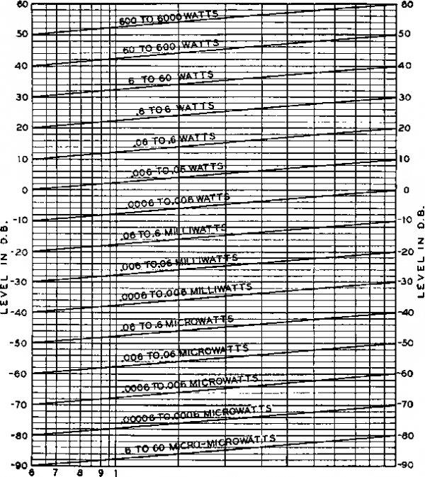

POWER

Figure 9.

CONVERSION CHART: POWER TO DECIBELS

Power levelt between 6 mlcromlereiwatt* and 6000 watt* пмгу be referred to eorretponding decibel levefs between -90 and 60 db, and vice verta, by meant ot the above chert. Fifteen ranges are provided. CocA curve beffini at tbe some point where the preceding one ends, enabllnff unliaerrupted coverage ot the wide db and power ranges with condensed chart. For example: the lowermost curve ends ot -SO db or 60 micromicrowotts and tbe next range ttortt ot the same leivel. Zero db feref 1%

taken as 6 mllllwaiU (.006 wait).

Converting Decibels to Power

It is often convenient to be able to convert a decibel value to a pow-er equivalent. The formula used for this operation is

P = 0.006 X antilog

Ndb 10

where P is the desired level in watts and Ndb the decibels to be converted.

To determine the power level P from a decibel equivalent, simply divide the decibel value by 10; then take the number comprising the antilog and multiply it by 0.006; the product gives the level in watts.

Note: In problems dealing with the conversion of min s decibels to power, it often happens that the decibel value -Мль is not divisible by 10. When this is the case.

the numerator in the factor -

must be

made evenly divisible by 10, the negative signs must be observed, and the quotient labeled accordingly.

To make the numerator evenly divisible by 10 proceed as follows: Assume, for example, that -Ndb is some such value as -38; to make this figure evenly divisible by 10, we must add -2 to it, and, since we have added a negative 2 to it, we must also add a positive 2 so as to keep the net result the same.

Our decibel value now stands, -40 + 2. Dividing both of these figures by 10, as in the equation above, we have - 4 and +0.2. Putting the two together we have the logarithm - 4.2 with the negative characteristic and the positive mantissa as required.

The following examples will show the technique to be followed in practical problems.

(a) The output of a certain device is rated at -74 db. What is the power equivalent? Solution:

= = <not evenly divisible by 10)

Routine:

-74 - 6

-80 +6

Hib -80 4- 6 10 - 10

= -8.6

antilog -8.6 = 0.000 ООО 04 .006 X 0.000 ООО 04 = 0.000 ООО ООО 24 wott or 240 micro-microwatt

(b) This example differs somewhat from that of the foregoing one in that the mantissas are added differently. A low-powered amphfier has an input signal level of -17.3 db. How many milliwatts does this value represent?

Solution:

-17.3 - 2.7

+ 2.7

Ndb -20 -f 2.7

+ 2.7 = -2.27

10 - 10 Antilog -2.27 == 0.0186

0.006 X 0.0186 = 0.000 1116 watt or 0.1116 milliwatt

Input voltages: To determine the required input voltage, take fhe peak voltage necessary to drive the last class A amplifier tube to maximum output, and divide this figure by the total overall voltage gain of the preceding stages.

Computing Specifications: From the preceding explanations the following data can be computed with any degree of accuracy warranted by the circumstances:

(1) Voltage amplification

(2) Overall gain in db

(3) Output signal level in db

(4) Input signal level in db

(5) Input signal level in watts

(6) Input signal voltage

When a power level is available which must be brought up to a new power level, the gain required in the intervening amplifier is equal to the difference between the two levels in decibels. If the required input of an amplifier for full output is -30 decibels and the output from a device to be used is but -45 decibels, the pre-amphfier required should have a gain of the difference, or 15 decibels. Again this is true only if the two amplifiers are properly matched and no losses are introduced due to mismatching.

Push-Pull To double the output of any cas-Amplifiers cade amplifier, it is only necessary to connect in push-pull the last amplifying stage, and replace the interstage and output transformers with push-pull types.

To determine the voltage gain (voltage ratio) of a push-pull amplifier, take the ratio of one half of the secondary winding of the push-pull transformer and multiply it by the /i of one of the output tubes in the push-pull stage; the product, when doubled, wi 1 be the voltage amplification, or step-up.

Other Units and Zero Levels

When working with decibels one should not immediately take for granted that the zero level is 6 milliwatts for there are other zero levels in use.

In broadcast stations an entirely new system is now employed. Measurements made iti

acoustics are now made with the standard zero level of 10 watts per square cm.

Microphones are often rated with reference to the following zero level: one volt at open circuit when the sound pressure is one millibar. In any case, the rating of the microphone must include the loudness of the sound. It is obvious that this zero level does not lend itself readily for the calculation of required gain in an amplifier.

The VU: So far, the decibel has always referred to a type of signal which can readily be measured, that is, a steady signal of a single frequency. But what would be the power level of a signal which is constantly varying in volume and frequency? The measurement of voltage would depend on the type of instrument employed, whether it is measured with a thermal square law meter or one that shows average values; also, the inertia of the movement will change its indications at the peaks and valleys.

After considerable consultation, the broadcast chains and the Bell System have agreed on the VU. The level in VU is the level in decibels above 1 milliwatt zero level and measured with a carefully defined type of instrument across a 600 ohm line. So long as we deal with an unvarying sound, the level in VU is equal to decibels above 1 milliwatt; but when the sound level varies, the unit is the VU and the special meter must be used. There is then no equivalent in decibels.

The Neper: We might have used the natural logarithm instead of the common logarithm when defining our logarithmic unit of sound. This was done in Europe and the unit obtained is known as the neper or napier. It is still found in some American literature on filters.

1 neper = 8.686 decibels 1 decibel = 0.1151 neper

AC Meters With Decibel Scales

Many test instruments are now equipped with scales calibrated in decibels which is very handy when making measurements of frequency characteristics and gain. These meters are generally calibrated for connection across a 500 ohm line and for a zero level of 6 milliwatts. When they are connected across another impedance, the reading on the meter is no longer correct for the zero level of 6 milliwatts. A correction factor should be applied consisting in the addition or subtraction of a steady figure to all readings on the meter. This figure is given by the equation:

db to be added = 10 log

where Z is the impedance of the circuit under measurement.

Figure 10. THE CIRCLE IS DIVIDED INTO FOUR QUADRANTS BY TWO PER-PENDICULAR LINES AT RIGHT ANGLES TO EACH OTHER. The ftortfieait quoilrant thus formed Is known as the first quadrant; tiie others are numbered eonseeutiveiy in a counterclockwise direction.

Trigonometry

Definition Trigonometry is the science of and Use mensuration of triangles. At first glance triangles may seem to have little to do with electrical phenomena; however, in a.c. work most currents and voltages follow laws equivalent to those of the various trigonometric relations which we are about to examine briefly. Examples of their application to a.c. work will be given in the section on Vectors.

Angles are measured In degrees or in radians. The circle has been divided into 360 degrees, each degree into 60 minutes, and each minute into 60 seconds. A decimal division of the degree is also in use because it makes calculation easier. Degrees, minutes and seconds are indicated by the following signs: and . Example: 6° 5 23 means six degrees, five minutes, twenty-three seconds. In the decimal notation we simply write 8.47°, eight and forty-seven hundredths of a degree.

When a circle Is divided into four quadrants by two perpendicular lines passing through the centet (Figure 10) the angle made by the two lines is 90 degrees, known as a right angle. Two right angles, or 180° equals a straight angle.

The radian: If we take the radius of a circle and bend it so it can cover a part of the circumference, the arc it covers subtends an angle called a radian (Figure 11). Since the circumference of a circle equals 2 times the radius, there are Itt radians in 360°. So we have the following relations:

1 radiants? 1745 = 57.2958° 7Г = 3.14159

1 degree=0.01745 radians

n-radians = 180° /2 radians=90 *

jr/3 radians = 60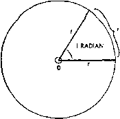

Figure 11. THE RADIAN.

A radian is an angle whose arc is exactly equal to the length of either side. Note thai ihe angle is constant regardless of ihe length of the side and the arc so long as they are equal. A radian equals 57.2958°.

In trigonometry we consider an angle generated by two lines, one stationary and the other rotating as if it were hinged at 0, Figure 12. Angles can be greater than 180 degrees and even greater than 360 degrees as illustrated in this iigure.

Two angles are complements of each other when their sumis 90°, or a right angle. A is the complement of В and В is the complement of A when

A=(90-B)

and when

B=(90-A)

Two angles are supplements of each other when their sum is equal toa straight angle, or 180°. A is the supplement of В and В is the supplement of A when

A = (180-B)

B = (180°-A)

In the angle A, Figure 13A, a line Is drawn from P, perpendicular fo b. Regardless of the point selected for P, the ratio a/c will always be the same for any given angle, A. So will all the other proportions between a, b, and с remain constant regardless of the position of point P on c. The six possible ratios each are named and defined as follows:

sine A = tangent A =

a с a

cosine A - -

cotangent A -

secant A =

cosecant A = - a

Let us take a special angle as an example. For instance, let the angle A be 60 degrees as in Figure 13B. Then the relations between the sides are as in the figure and the six functions become:

sin. 60° = - =

cos 60° = = 1/2

tan 60° =

cot 60° =

sec 60° = = = 2 b Уг

CSC 60° - ~ a

= /3

Уг JL Угъ VI

Угъ

= УъуГъ

Another example: Let the angle be 45°, then the relations between the lengths of a, b, and с are as shown in Figure 13Q and the six functions are: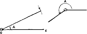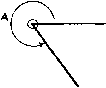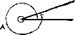

Figure 12.

AN ANGLE IS GENERATED BY TWO LINES, ONE STATIONARY AND THE OTHER

ROTATING.

The line OX is stationary; the line with the small arrow at the far end rotates in a counterclocliwise direction. At the position illustrated in the lefthandmost section of the drawing it mofces an angle, A, which is less than 90° ond is therefore in the first quadrant. In the position shown in the second portion of the drawing the angle A has Increased to such a value tltat it now lies in the third quadrant; note that an angle can be greater than 780°. In the third illustration the angle A is In the fourth quadrant. In the fourth position the rotating vector has made more than one complete revolution and is hence in ihe fifth quadrant; since ihe fifth quadrant is an exact repetition of th first quadrant, its values will be ihe some as In the lefthandmost portion of ihe Illustration.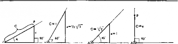

b = 0

®

Figure 1 3. THE TRIGONOMETRIC FUNCTIONS.

In the right triangle shown in (A) the side opposite the angle A is a, while the adjoiniitg sides are b and e; the trigonometric functions of the angle A are completely defined by the ratios of the sides a, b and c. In (B) are shown the lengths of the sides a and b when angle A is M and side с is 7. In (C) angle A is 45°; a and b equal 7, while с equals л/2. In (D) note that с equafs a for a

right angle while b equals 0.

sin ~ = 1/, VI

cos 45° = i/2V

tan 45° sec 45°

cot 45° = - = 1

VY r-

cosec45° = f-= Vl

There are some special difficulties when the angle is zero or 90 degrees. In Figure 13D an angle of 90 degrees is shown; drawing a line perpendicular to h from point P makes it fall on top of c. Therefore in this case a - с and b - Q. The six ratios are now:

-= 1

sin 90° -

tan 90° -1-=-=

. b 0 cos 90° --- - 0

cot 90° = -= 0 a

sec90° =4 = -= °° cosec90°= -=1 bo \ a

When the angle is zero, d = 0 and b - c. The

values are then:

. a 0 sm0° = -=-= 0

tan 0° = = A = 0 b b

cos0° = -= 1

cot 0=

b 0

sec 0° 1

с с

cosec 0° = -=77= °° a 0

In general, for every angle, there will be definite values of the six functions. Conversely, when any of the six functions is known, the angle is defined. Tables have been calculated giving the value of the functions for angles.

From the foregoing we can make up a small table of our own (Figure 14), giving values of the functions for some common angles.

Relations Between Functions

sin A =

It follows from the definitions that

cosec A and tan A =

cos A = 1

sec A

cot A

From the definitions also follows the relation

cos A = sin (complement of A)=sin (90°-A)

because in the right triangle of Figure 15, cos A = b/c = sinB and B = 90°-A or the complement of A. For the same reason:

cot A = tan (90°-A) CSC A = sec (90°-A)

Relations in Right Triangles

In the right triangle of Figure 15, un A=a/c and by transposition

a = с sin A

For the same reason we have the following identities:

tan A = a/b cot A = b/a

a = b tan A b = a cot A

In the same triangle we can do the same for functions of the angle E

Angle Sin Cos. Tan Cot Sec. Cosec.

0 0 1 0 > 1

30° 1/2 i/zVlVsVT Vb 2

45° 1/2 V2 1/2/2 1 I Vl Vl

60° 1/2V3 1/2 Vb ViVb 2 2/3vT

90° 1 0 CO 0 00 1 Figure 14.

Values of trigonometric functions for common angles in the first quadrant.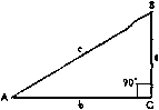

POSITIVE FUNCTIONS

SECOND QUADRANT FIRST OUADRaNT

tine, cosec

Figure 15.

In this figure the sides a, b, and e are used to define the trigonometric functions of angle В as well as angle A.

Functions of Angles Greater than 90 Degrees

In angles greater than 90 degrees, the values of a and h become negative on occasion in accordance with the rules of Cartesian coordinates. When I) is measured from 0 towards the left it is considered negative and similarly, when a is measured from 0 downwards, it is negative. Referring to Figure 16, an angle in the second quadrant (between 90° and 180°) has some of its functions negative:

= pos. COS A =

all functions

THIRD (?UADRANT FOURTH OUADRANT

Figure 17.

SIGNS OF THE TRIGONOMETRIC FUNCTIONS.

The functions listed in this diagram are posi-tive; all other functions are negative.

sec A = = neg.

cosec A = neg.

sin A = -- =

cot A =

с

с

- neg.

= neg.

And in the fourth quadrant (270° to 360°):

tan A = = neg.

sec A = = neg. cosec A = = pos

For an angle in the third quadrant (180° to 270°), the functions are

sin A = - = neg. cos A =- - neg.

cot A = = pos.

. -a tan A = -JT- = pos.

Summarizing, the sign of the functions in each quadrant can be seen at a glance from Figure 17, where in each quadrant are written the names of functions which are positive; those not mentioned are negative.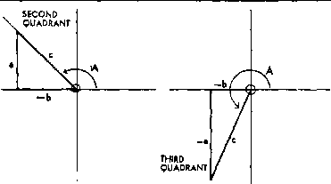

Figure 16.

TRIGONOMETRIC FUNCTIONS IN THE SECOND, THIRD, AND FOURTH QUADRANTS.

TAe trigonometric functions In these quadrants are similar to first quadrant values, but the Signs of the functions vary as listed In the text and in figure 17.

Figure IS. SINE AND COSINE CURVES.

In (Л) we have a sine curve drown in Cartesian coordinates. This is the usual representation of an alternating current wave without substantial harmonics. In (B) we have a cosine wave; note that it is exactly similar to a sine wave displaced by 90° or n/2 radians.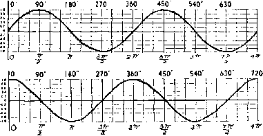

Graphs of Trigonometric Functions

The sine nave. When we have the relation y - sinx, where x is an angle measured in radians or degrees, we can draw a curve of у versus x for all values of the independent variable, and thus get a good conception how the sine varies with the magnitude of the angle. This has been done in Figure isA. We can learn from this curve the following facts.

1. The sine varies between +1 and - i

2. It is a periodic curve, repeating itself after every multiple of 27г or 360°

3. Sin X = sin (180° -x) or sin ( гг - x)

4. Sin x = -sin (180° + x). or - sin (тг + x)

The cosine leave. Making a curve for the function у = cos x, we obtain a curve similar to that for у = sin X except that it is displaced by 90° or П-/2 radians with respect to the Y-axis. This curve (Figure 18B) is also periodic but it does not start with zero. We read from the curve:

1. The value of the cosine never goes beyond + 1 or -1

2. The curve repeats, after every multiple of 2-77 radians or 360°

3. Cos X - -cos (180° -x) or

- cos ( - x)

4. Cos x - cos (360° -x) or cos (2- -x) The graph of the tangent is illustrated in

Figure 19. This is a discontinuous curve and illustrates well how the tangent increases from zero to infinity when the angle increases from zero to 90 degrees. Then when the angle is further increased, the tangent starts from minus infinity going to zero in the second quadrant, and to infinity again in the third quadrant.

1. The tangent can have any value between + 0= and - 0=

2. The curve repeats and the period is ir radians or 180°, not 27г radians

3. Tan X = tan (180° 4-х) or tan (ir+x)

4. Tan X ~ -tan (180° -x) or

- tan (-tt -x)

The graph of the cotangent is the inverse of that of the tangent, see Figure 20. It leads us to the following conclusions:

1. The cotangent can have any value between + ra and - ra

2. It is a periodic curve, the period being TT radians or 180°

3. Cot X = cot (180° -bx) or cot (тг +x)

4. Cot X = -cot (180° -x) or -cot {rr -x)

90°

270°

450°

630°

Figure 19. TANGENT CURVES.

The tangent curve increases from 0 to ra an angular increase of 90°. In the next it increases from -a> to + od .

with 780°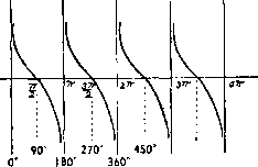

630 540° 7го*

Figure 20. COTANGENT CURVES.

Cotongent curves ore the Inverse of the tangent curves. They vary from + m to - a> In each pair of iuadrants.

COTANGENT.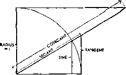

COSINE

Figure 21. ANOTHER REPRESENTATION OF TRIGONOMETRIC FUNCTIONS.

If the radius of a circle is considered as the unit of measurement, then the lengths of the yariaus lines shown in this diagram are numerically equal ta the functions marked adjacent to them.

The graphs of the secant and cosecant are of lesser importance and will not be shown here. They are the inverse, respectively, of the cosine and the sine, and therefore they vary from +1 to infinity and from -1 to -infinity.

Perhaps another useful way of visualizing the values of the functions is by considering Figure 21. If the radius of the circle is the unit of measurement then the lengths of the lines are equal to the functions marked on them.

Trigonometric Tables There are two kinds of

trigonometric tables. The first type gives the functions of the angles, the second the logarithms of the functions. The first kind is also known as the table of natural trigonometric functions.

These tables give the functions of all angles between 0 and 45°. This is all that is necessary for the function of an angle between 45° and 90° can always be written as the co-function of an angle below 45°. Example: If we had to find the sine of 48°, we might write

sin 48°= cos (90° -48°)= cos 42°

Tables of the logarithms of trigonometric functions give the common logarithms (logw) of these functions. Since many of these logarithms have negative characteristics, one should add -10 to ail logarithms in the table which have a characteristic of 6 or higher. For instance, the log sin 24° = 9-60931 -10. Log tan 1° = 8.24192 -10 but log cot 1° = 1.75808. When the characteristic shown is less than 6, it is supposed to be positive and one should not add -10.

Vectors

A scalar quantity has magnitude only; a vector quantity has both magnitude and direction. When we speak of a speed of 50 miles per hour, we are using a scalar quantity, but when we say the wind la Northeast and has a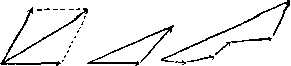

Figure 22.

Vectors may be added as shown in these sketches. In each case the long vector represents the vector sum of the smaller vectors. For many engineering applications sufficient accuracy can be obtained by this method which avoids long and laborious calculations.

velocity of 50 miles per hour, we speak of a vector quantity.

Vectors, representing forces, speeds, displacements, etc., are represented by arrows. They can be added graphically by well known methods illustrated in Figure 22. We can make the parallelogram of forces or we can simply draw a triangle. The addition of many vectors can be accomphshed graphically as in the same figure.

In order that we may define vectors algebraically and add, subtract, multiply, or divide them, we must have a logical notation system that lends itself to these operations. For this purpose vectors can be defined by coordinate systems. Both the Cartesian and the polar coordinates are in use.

Vectors Defined by Cartesian Coordinates

Since we have seen how the sum of two vectors is obtained, it follows from Figure 23, that the vector Z equals the sum of the two vectors x and y. In fact, any vector can be resolved into vectors along the X- and У-axis. For convenience in working with these quantities we need to dis-

Figure 23.

RESOLUTION OF VECTORS.

Any vector such as Z may be resolved into two vectors, X and y, along the X- and Y-axes. If vectors are to be added, their respective X and у components may be added to find the X and у components of (be reswf(an( vector.