HANDBOOK

Vectors 771

Figure 24. ADDITION OR SUBTRACTION OF VECTORS.

Vector* moy be added or subtracted by adding or subtracting their x or у components separately.

tinguish between the X- and V-component, and so it has been agreed that the V-component alone shall be marked with the letter /. Example (Figure 23):

Z = 3 + 4j

Note again that the sign of components along the X-axis is positive when measured from 0 to the right and negative when measured from 0 towards the left. Also, the component along the V-axis is positive when measured from 0 upwards, and negative when measured from 0 downwards. So the vector, R, is described as

R = 5 - 3i

Vector quantities are usually indicated by some special typography, especially by using a point over the letter indicating the vector, as

Absolute Value of a Vector

The absolute or scalar value of vectors such as Z

or R in Figure 23 is easily found by the theorem of Pythagoras, which states that in any right-angled triangle the square of the side opposite the right angle is equal to the sum of the squares of the sides adjoining the right angle. In Figure 23, OAB is a right-angled triangle; therefore, the square of OB (or Z) is equal to the square of OA (or x) plus the square of AB (or y). Thus the absolute values of Z and R may be determined as fohows:

Z Z R

= V 5 + 3 = / 34 = 5.83

The vertical lines indicate that the absolute or scalar value is meant without regard to sign or direction.

Addition of Vectors

the two vectors

An examination of Figure 24 will show that

R = Xl + j yi Z = X, -t- j y,

can be added, if we add the X-components and the V-components separately.

R -b Z = Xl -t- X, + i (y. + y,)

For the same reason we can carry out subtraction by subtracting the horizontal components and subtracting the vertical components

R - Z = Xl - X2 + j (yi - ys)

Let us consider the operator /, If we have a vector a along the X-axis and add a ; in front of it (multiplying by /) the result is that the direction of the vector is rotated forward 90 degrees. If we do this twice (multiplying by f) the vector is rotated forward by 180 degrees and now has the value -a. Therefore multiplying by f is equivalent to multiplying by -1. Then

f = - 1 and j = V - 1

This is the imaginary number discussed before under algebra. In electrical engineering the letter / is used rather than i, because i is already known as the symbol for current.

Multiplying Vectors When two vectors are

to be multiplied we can perform the operation just as in algebra, remembering that j = -l.

RZ = (x, + jyi) (x, + jy,)

= Xl X2 + jXl У2 + j X2 yi + f yi У2 = Xl Xs - yi У2 + j (Xi Уг + X2 yi)

Division has to be carried out so as to remove the /-term from the denominator. This can be done by multiplying both denominator and numerator by a quantity which will eliminate ; from the denominator. Example:

R 1 + jyi (Xi + jyi) (X2 - уг)

2 ~ 5 + iy ~ ( 2 + jyi) (X2 - jya)

XiX2 + yiyg + j (Xayi - Xiya)

Polar Coordinates A vector can also be defined in polar coordinates by its magnitude and its vectorial angle with an arbitrary reference axis. In Figure 25

Figul-e 25 IN THIS FIGURE A VECTOR HAS BEEN REPRESENTED IN POLAR INSTEAD OF CARTESIAN COORDINATES. In polar coordinates a vector is defined by a magnitude and an angle, called the vectorial angle, instead of by two magnitudes as in Cartesian coordinates.

the vector Z has a magnitude 50 and a vectorial angle of 60 degrees. This will then be written

Z = 50/60°

A vector a + jb can be transformed into polar notation very simply (see Figure 26)

Z = a -bib = Va= -b

b /Юп I

In this connection tan means the angle of which the tangent is. Sometimes the notation arc tan b/a is used. Both have the same meaning.

A polar notation of a vector can be transformed into a Cartesian coordinate notation in the following manner (Figure 27)

Z = p/A = p cos A -f- jp sin A

A sinusoidally alternating voltage or current is symbolically represented by a rotating vector, having a magnitude equal to the peak voltage or current and rotating with an angular velocity of 277f radians per second or as many revolutions per second as there are cycles per second.

The instantaneous voltage, e, is always equal to the sine of the vectorial angle of this rotating vector, multiplied by its magnitude.

e = E sin 27rft

The alternating voltage therefore varies with time as the sine varies with the angle. If we plot time horizontally and instantaneous voltage vertically we will get a curve like those in Figure 18.

In alternating current circuits, the current

TAN A=

Figure 26. Vectors can be transformed from Cartesian into polar notation as shown in this figure.

which flows due to the alternating voltage is not necessarily in step with it. The rotating current vector may be ahead or behind the voltage vector, having a phase difference with it. For convenience we draw these vectors as if they were standing still, so that we can indicate the difference in phase or the phase angle. In Figure 28 the current lags behind the voltage by the angle $, or we might say that the voltage leads the current by the angle 6.

Vector diagrams show the phase relations between two or more vectors (voltages and currents) in a circuit. They may be added and subtracted as described; one may add a voltage vector to another voltage vector or a current vector to a current vector but not a current vector to a voltage vector (for the same reason that one cannot add a force to a speed). Figure 28 illustrates the relations in the simple series circuit of a coil and resistor. We know that the current passing through coil and resistor must be the same and in the same phase, so we draw this current / along the X-axis. We know also that the voltage drop IR across the resistor is in phase with the current, so the vector IR representing the voltage drop is also along the X-axis.

The voltage across the coil is 90 degrees ahead of the current through it; IX must therefore be drawn along the У-axis. E the applied voltage must be equal to the vectorial sum of the two voltage drops, IR and IX, and we have so constructed it in the drawing. Now expressing the same in algebraic notation, we have

E = IR -I- ilX

Dividing by /

IZ = IR -b ilX

Z = R -h iX

Due to the fact that a reactance rotates the voltage vector ahead or behind the current vector by 90 degrees, we must mark it with a / in vector notation. Inductive reactance will have a plus sign because it shifts the voltage vector forwards; a capacitive reactance is neg-

1 p SIN A

pCOSA

Figure 27.

Vectors can be iransforrned from polar into Cartesiari riotatiori as shown in this figure.

ative because the voltage will lag behind the current. Therefore:

X, = + i 2;7fL 1

Xo = - i

2ittC

In Figure 28 the angle в is known as the phase angle between E and I. When calculating power, only the real components count. The power in the circuit is then

P = I (IR)

but IR = E cos в

.. P = El cos 9

This cos 9 is known as the power factor of the circuit. In many circuits we strive to keep the angle в as small as possible, making cos 9 as near to unity as possible. In tuned circuits, we use reactances which should have as low a power factor as possible. The merit of a coil or condenser, its Q, is defined by the tangent of this phase angle:

Q = ton e = X/R

For an efficient coil or condenser, Q should be as large as possible; the phase-angle should then be as close to 90 degrees as possible, making the power factor nearly zero. Q is almost but not quite the inverse of cos в. Note that in Figure 29

Q =X/R and cos в = R/Z

When Q is more than 5, the power factor is less than 20%; we can then safely say Q - 1/cos в with a maximum error of about 2У2 percent, for in the worst case, when cos в = 0.2, Q will equal tan 9 = 4.89- For higher values of Q, the error becomes less.

Note that from Figure 29 can be seen the simple relation:

Z = R + jXi

Z = V + Xi,

Figure 28. VECTOR REPRESENTATION OF A SIMPLE SERIES CIRCUIT.

The righihand portion af the illustration shows the vectors representing the voltage drops in the coil and resistance illustrated at the left. Note that the voltage drop across the coil Xl leads that across the resistance by 90 .

Graphicol Representation

Formulas and physical laws are often presented in graphical form; this gives us a birds eye view of various possible conditions due to the variations of the quantities involved. In some cases graphs permit us to solve equations with greater ease than ordinary algebra.

Coordinate Systems All of us have used coordinate systems without realizing it. For instance, in modern cities we have numbered streets and numbered avenues. By this means we can define the location of any spot in the city if the nearest street crossings are named. This is nothing but an apphcation of Cartesian coordinates.

In the Cartesian coordinate system (named after Descartes), we define the location of any point in a plane by giving its distance from each of two perpendicular lines or axes. Figure 30 illustrates this idea. The vertical axis is called the Y-axis, the horizontal axis is the X-axis. The intersection of these two axes is called the origin, 0. The location of a point, P, (Figure 30) is defined by measuring the respective distances, x and у along the X-axis and the Y-axis. In this example the distance along the X-axis is 2 units and along the Y-axis is 3 units. Thus we define the point as

POWER FACTOR=COS в=

Figure 29.

The figure of merit of a coil and Its resistance is represented by the ratio of the inductive reactance to the resistance, which as shown

in this diagram is equal to which equafs

tan e. For forge values of в (the phase angle) this is approximately equal to the reciprocal of the cos Q.

Figure 30. CARTESIAN COORDINATES.

The location ot any point can be defined by its distance from the X and Y axes.

P 2, 3 or we might say x = 2 and у ~ 3. The measurement x is called the abscissa of the point and the distance у is called its ordinate. It is arbitrarily agreed that distances measured from 0 to the right along the X-axis shall be reckoned positive and to the left negative. Distances measured along the l:-axis are positive when measured upwards from 0 and negative when measured downwards from 0. This is illustrated in Figure 30. The two axes divide the plane area into four parts called quadrants. These four quadrants are numbered as shown in the figure.

It follows from the foregoing statements, that points lying within the first quadrant have both X and у positive, as is the case with the point P. A point in the second quadrant has a negative abscissa, x, and a positive ordinate, y. This is illustrated by the point Q, which has the coordinates x = -4 and у = +1. Points in the third quadrant have both x and у negative. X = - 5 and у - -2 illustrates such a joint, R. The point S, in the fourth quadrant las a negative ordinate, у and a positive abscissa or X.

In practical applications we might draw only as much of this plane as needed to illustrate our equation and therefore, the scales along the X-axis and Y-axls might not start with zero and may show only that part of the scale which interests us.

Representation of Functions

In the equation:

Ikc 600

Figure 31.

REPRESENTATION OF A SIMPLE FUNCTION IN CARTESIAN COORDINATES.

300,000

In this chart of the function fkc = т-

distances along the X axis represent wavelength in meters, while those along the Y axis represent frequency in liilocycles. A curve such as this helps to find values between those calculated with sufficient accuracy for most purposes.

f is said to be a function of X. For every value of / there is a definite value of X. A variable is said to be a funcrion of another variable when for every possible value of the latter, or independent variable, there is a definite value of the first or dependent variable. For instance, if у = 5x J is a function of x and x is called the independent variable. When a = 3b + 5b - 25b + б then d is a function of b.

A function can be illustrated in our coordinate system as follows. Let us take the equation for frequency versus wavelength as an example. Given difierent values to the independent variable find the corresponding values of the dependent variable. Then plot the points represented by the different sets of two values.

Plotting these points in Figure 31 and drawing a smooth curve through them gives us the curve or graph of the equation. This curve will help us find values of / for other values of X (those in between the points calculated) and so a curve of an often-used equation may serve better than a table which always has gaps.

When using the coordinate system described so far and when measuring linearly along both axes, there are some definite rules regarding

HANDBOOK

Representation of Functions 775

Figure 32.

Only two points are needed to define functions which result in a siraigtit line as shown in this diagram representing Ohms Law.

the kind of curve we get for any type of equation. In fact, an expert can draw the curve with but a very few plotted points since the equation has told him what kind of curve to expect.

First, when the equation can be reduced to the form у = mx + b, where x and у are the variables, it is known as a linear or first degree function and the curve becomes a straight line. (Mathematicians still speak of a curve when it has become a straight line.)

When the equation is of the second degree, that is, when it Contains terms like or У or xy, the graph belongs to a group of curves, called conic sections. These include the circle, the ellipse, the parabola and the hyperbola. In the example given above, our equation is of the form

xy = c, с being equal to 300,000

which is a second degree equation and in this case, the graph is a hyperbola.

This type of curve does not lend itself readily for the purpose of calculation except near the middle, because at the ends a very large change in \ represents a small change in / and vice versa. Before discussing what can be done about this let us look at some other types of curves.

Suppose we have a resistance of 2 ohms and we plot the function represented by Ohms Law: E ~ 21. Measuring £ along the X-axis and amperes along the V-axis, we plot the necessary points. Since this is a first degree equation, of the form у = mx -h b (for E = y, m - 2 and I - x and b - 0) it will be a straight line so we need only two points to plot it.

(line passes through origin) q 0

5 10

The line is shown in Figure 32. It is seen to be a straight line passing through the origin.

Figure 33. A TYPICAL GRID - VOLTAGE PLATE-CURRENT CHARACTERISTIC CURVE.

The equation represented by such a curve Is so complicated thai we do not use ii. Data for such a curve is obtained experimentally, and intermediate values can be found with suttieient accuracy from the curve.

li the resistance were 4 ohms, we should get the equation E = 41 and this also represents a line which we can plot in the same figure. As we see, this line also passes through the origin but has a different slope. In this illustration the slope defines the resistance and we could make a protractor which would convert the angle into ohms. This fact may seem inconsequential now, but use of this is made in the drawing of loadhnes on tube curves.

Figure 33 shows a typical, grid-voltage, plate-current static characteristic of a triode. The equation represented by this curve is rather complicated so that we prefer to deal with the curve. Note that this curve extends through the first and second quadrant.

Families of curves. It has been explained that curves in a plane can be made to illustrate the relation between two variables when one of them varies independently. However, what are we going to do when there are three variables and two of them vary independently. It is possible to use three dimensions and three axes but this is not conveniently done. Instead of this we may use a family of curves. We have already illustrated this partly with Ohms Law. If we wish to make a chart which will show the current through any resistance with any voltage applied across it, we must take the equation E = IR, having three variables.

We can now draw one line representing a resistance of 1 ohm, another line representing 2 ohms, another representing 3 ohms, etc., or as many as we wish and the size of our paper will allow. The whole set of lines is then applicable to any case of Ohms Law falling within the range of the chart. If any two of the three quantities are given, the third can be found.

AVERASE PLATE CHARACTERISTICS E!=6,3 V.

Figure 34. A FAMILY OF CURVES. An equation such as Ohms Law has three variables, but can be represented in Cartesian coordinates by a family of curves such as shown here. If any two quantities are given, the third can be found. Any point in the chart represents a definite .value each of E, /, and R, which will satisfy the equation oil Ohms Law. Values of R not situated oa an R line can be found by interpolation.

Figure 34 shows such a family of curves to solve Ohms Law. Any point in the chart represents a definite value each of E, I, and R which will satisfy the equation. The value of R represented by a point that is not situated on an R hne can be found by interpolation.

It is even possible to draw on the same chart a second family of curves, representing a fourth variable. But this is not always possible, for among the four variables there should be no more than two independent variables. In our example such a set of lines could represent power in watts; we have drawn only two of these but there could of course be as many as desired. A single point in the plane now indicates the four values of E, I, R, and P which belong together and the knowledge of any two of them will give us the other two by reference to the chart.

Another example of a family of curves is the dynamic transfer characteristic or plate family of a tube. Such a chart consists of several curves showing the relation between plate voltage, plate current, and grid bias of a tube. Since we have again three variables, we must show several curves, each curve for a fixed value of one of the variables. It is customary to plot plate voltage along the X-axis, plate current along the У-axis, and to make different curves for various values of erid bias. Such a

no Ht 3

PUrrr WLTett-VeiTS

Figure 35. PLATE CURVES FOR A TYPICAL VACUUM TUBE. /II such curves we have three variables, plate voltage, plate current, and grid bias. Each point on a grid bias line corresponds to the plate voltage and plate current represented by its position with respect to the X and Y axes. Those for other values of grid bias may be found by interpolation. The loadline shown in the lower left portion of the chart is ex-plairted in the text.

set of curves is illustrated in Figure 35. Each point in the plane is defined by three values, which belong together, plate voltage, plate current, and grid voltage.

Now consider the diagram of a resistance-coupled amplifier in Figure 36. Starting with the B-supply voltage, we know that whatever plate current flows must pass through the resistor and will conform to Ohms Law. The voltage drop across the resistor is subtracted from the plate supply voltage and the remainder is the actual voltage at the plate, the kind that is plotted along the X-axis in Figure 35. We can now plot on the plate family of the

Figure 36. PARTIAL DIAGRAM OF A RESISTANCE COUPLED AMPLIFIER. The portion of the supply voltage wasted across the 50,000-ohm resistor is represented In figure 35 as tlie loadline.

HANDBOOK

Logarithmic Scales 777

tube the loadline, that is the line showing which part of the plate supply voltage is across the resistor and which part across the tube for any value of plate current. In our example, let us suppose the plate resistor is 50,000 ohms. Then, if the plate current were zero, the voltage drop across the resistor would be zero and the full plate supply voltage is across the tube. Our first point of the loadline is £ = 250, 7 = 0. Next, suppose, the plate current were 1 ma., then the voltage drop across the resistor would be 50 volts, which would leave for the tube 200 volts. The second point of the load-line is then £ = 200, / = 1. We can continue like this but it is unnecessary for we shall find that it is a straight line and two points are sufficient to determine It.

This loadline shows at a glance what happens when the grid-bias is changed. Although there are many possible combinations of plate voltage, plate current, and grid bias, we are now restricted to points along this hne as long as the 50,000 ohm plate resistor is in use. This line therefore shows the voltage drop across the tube as well as the voltage drop across the load for every value of grid bias. Therefore, if we know how much the grid bias varies, we can calculate the amount of variation in the plate voltage and plate current, the amplification, the power output, and the distortion.

Logarithmic Scales Sometimes it is convenient to measure along the axes the logarithms of our variable quantities. Instead of actually calculating the logarithm, special paper is available with logarithmic scales, that is, the distances measured along the axes are proportional to the logarithms of the numbers marked on them rather than to the numbers themselves.

There is semi-logarithmic paper, having logarithmic scales along one axis only, the other scale being linear. We also have full logarithmic paper where both axes carry logarithmic sea es. Many curves are greatly simplified and some become straight lines when plotted on this paper.

As an example let us take the wavelength-frequency relation, charted before on straight cross-section paper.

300,000

Taking logarithms:

log i = lag 300,000 - log \

If we plot log / along the V-axis and log X along the X-axis, the curve becomes a straight line. Figure 37 illustrates this graph on full logarithmic paper. The graph may be read with the same accuracy at any point in con-

3000 2500

2000 1500

1000 900 800

700 600

>-

2 100

8 8

WAVELENGTH IN METERS

8 8 8 I

e 2

Figure 37. A LOGARITHMIC CURVE.

Atony functions become greatly simplified and some become straight lines when plotted to logarithmic scales such as shown in this diagram. Here the frequency versus wavelength curve of Figure 31 has iieen replotted to conform with logarithmic axes. Nate that it is only necessary to calculate two points in order to determine the curve since this type of function results in a straight line.

trast to the graph made with linear coordinates.

This last fact is a great advantage of logarithmic scales in general. It should be clear that if we have a linear scale with 100 small divisions numbered from 1 to 100, and if we are able to read to one tenth of a division, the possible error we can make near 100, way up the scale, is only 1/lOth of a percent. But near the beginning of the scale, near 1, one tenth of a division amounts to 10 percent of 1 and we are making a 10 percent error.

In any logarithmic scale, our possible error in measurement or reading might be, say 1/32 of an inch which represents a fixed amount of the log depending on the scale used. The net result of adding to the logarithm a fixed quantity, as 0.01, is that the anti-logarithm is multiplied by 1.025, or the error is 21/2%. No matter at what part of the scale the 0.01 is added, the error is always 21/2%-

An example of the advantage due to the use

10,000

10 5 0 5 10 15 KC. OFF RESONANCE

Figure 38. A RECEIVER RESONANCE CURVE. This curve represents the output of a receiver versus frequency when plotted to linear

coordinates.

of semi-logarittimic paper is shown in Figures 38 and 39. A resonance curve, when plotted on linear coordinate paper will look like the curve in Figure 38. Here we have plotted the output of a receiver against frequency while the applied voltage is kept constant. It is the kind of curve a wobbulator will show. The curve does not give enough information in this form for one might think that a signal 10 kc. off resonance would not cause any current at all and is tuned out. However, we frequently have off resonance signals which are 1000 times as strong as the desired signal and one cannot read on the graph of Figure 38 how much any signal is attenuated if it is reduced more than about 20 times.

In comparison look at the curve of Figure 39. Here the response (the current) is plotted in logarithmic proportion, which allows us to plot clearly how far off resonance a signal has to be to be reduced 100, 1,000, or even 10,000 times.

Note that this curve is now upside down ; it is therefore called a selectivity curve. The reason that it appears upside down is that the method of measurement is different. In a selectivity curve we plot the increase in signal voltage necessary to cause a standard output off resonance. It is also possible to plot this increase along the У-axis in decibels; the curve then looks the same although linear paper can

3 о

<

о о

cc О

< z

Й

LU К

<

о

э

о о

1000

КС. OFF RESONANCE

Figure 39. А RECEIVER SELECTIVITY CURVE.

This curve represents the selectivity of a receiver plotted to logarithmic coordinates for the output, but linear coordinates for frequency. The reason that this curve appears inverted from tbat of figure 38 is explained in the text.

be used because now our unit is logarithmic.

An example of full logarithmic paper being used for families of curves is shown in the reactance charts of Figures 40 and 41.

Nomograms or Alignment Charts

An alignment chart consists of three or more sets of scales which have been so laid out that to solve the formula for which the chart was made, we have but to lay a straight edge along the two given values on any two of the scales, to find the third and unknown value on the third scale. In its sim-

Figure 40.

REACTANCE-FREQUENCY CHART FOR AUDIO FREQUENCIES

See text for applicationi and instructions for use.

i i г

о о

Ч

I i я я л ял I ш .т А- № л

1 к к lb я ..т; I к я U к'<№ лял'.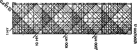

100 МС.

.V i.OJUHY 0.1

.001HY \ 100JJHY f 10JUHY .V i.OJUHY O.IJUHY .01JUHY

г к о ГАЧ ТЛЯ

Ю1 HY 10 МС.

100 MC.

KWM

ii;iiKa: .v.i:vaMii;iR KO( ;ft>r WK

ю ак1км 1 Т4

10 MC.

0>

шшш^шшшшштшгтшш

IMC.

1 HY

100 KCj

1000000 л

10000.0.

1000 п. Figure 41.

100 й

REACTANCE-FREQUENCY CHART FOR R.F.

This chart is used in conjunction with the nomograph on page 569 for radio frequency tonk coil computations.