 |
 |
 |
| Главная Журналы Популярное Audi - почему их так назвали? Как появилась марка Bmw? Откуда появился Lexus? Достижения и устремления Mercedes-Benz Первые модели Chevrolet Электромобиль Nissan Leaf |
Главная » Журналы » Metal oxide semiconductor 1 ... 64 65 66 67 68 69 70 ... 91 Motor Drives M. R Rahman, Ph.D. School of Electrical Engineering and Telecommunications, The University of New South Wales, Sydney, NSW 2052, Australia D. Patterson, Ph.D. Northern Territory Centre for Energy Research, Faculty of Technology, Northern Territory University, Darwin, NT 0909, Australia A. Cheok, Ph.D. Department of Electrical and Computer Engineering, National University of Singapore, 10 Kent Ridge Crescent, Singapore 119260 R. Betts, Ph.D. Department of Electrical and Computer Engineering, University of Newcastle, Callaghan, NSW 2308, Australia Introduction...................................................................................... 664 Dc Motor Drives................................................................................ 665 27.2.1 Introduction 27.2.2 DC Motor Representation and Characteristics 27.2.3 Converters for dc Drives 27.2.4 Drive System Integration 27.2.5 Converter-dc Drive System Considerations 27.2.6 Further Reading Induction Motor Drives....................................................................... 670 27.3.1 Introduction 27.3.2 Steady-State Representation 27.3.3 Characteristics and Methods of Control 27.3.4 Vector Controls 27.3.5 Further Reading Synchronous Motor Drives................................................................... 681 27.4.1 Introduction 27.4.2 Steady-State Equivalent-Circuit Representation of the Motor 27.4.3 Performance with Voltage Source Drive 27.4.4 Characteristics under Current-Source Inverter (CSI) Drive 27.4.5 Brushless dc Operation of the CSI Driven Motor 27.4.6 Operating Modes 27.4.7 Vector Controls 27.4.8 Further Reading Permanent Magnet ac Synchronous Motor Drives.................................... 689 27.5.1 Introduction 27.5.2 The Surface-Magnet Synchronous Motor 27.5.3 The PM Sine-Wave Motor 27.5.4 Further Reading Permanent-Magnet Brushless dc (BLDC) Motor Drives............................ 694 27.6.1 Machine Background 27.6.2 Electronic Commutation 27.6.3 Current/Torque Control 27.6.4 A Complete Controller 27.6.5 Summary 27.6.6 Further Reading Servo Drives...................................................................................... 704 27.7.1 Introduction 27.7.2 Servo-Drive Performance Criteria 27.7.3 Servo Motors, Shaft Sensors, and Coupling 27.7.4 The Inner Current/Torque Loop 27.7.5 Sensors for Servo Drives 27.7.6 Servo Control-Loop Design Issues 27.7.7 Further Reading Stepper Motor Drives.......................................................................... 710 27.8.1 Introduction 27.8.2 Motor Types and Characteristics 27.8.3 Mechanism of Torque Production 27.8.4 Single- and Multistep Responses 27.8.5 Drive Circuits 27.8.6 Microstepping 27.8.7 Open-Loop Acceleration-Deceleration Profiles 27.8.8 Further Reading Switched-Reluctance Motor Drives........................................................ 717 27.9.1 Introduction 27.9.2 Advantages and Disadvantages of Switched Reluctance Motors 27.9.3 Switched-Reluctance Motor Variable-Speed Drive Apphcations 27.9.4 SR Motor and Drive Design Options 27.9.5 Operating Theory of the Switched-Reluctance Motor: Linear Model 27.9.6 Operating Theory of the SR Motor (11): Magnetic Saturation and Nonlinear Model 27.9.7 Control Parameters of the SR Motor 27.9.8 Position Sensing 27.9.9 Further Reading 27.10 Synchronous Reluctance Motor Drives................................................. 727 27.10.1 Introduction 27.10.2 Basic Principles 27.10.3 Machine Structure 27.10.4 Basic Mathematical Modeling 27.10.5 Control Strategies and Important Parameters 27.10.6 Practical Considerations 27.10.7 A Syncrel Drive System 27.10.8 Conclusions References.......................................................................................... 733 27.1 27.2 27.3 27.4 27.5 27.6 27.7 27.8 27.9 27.1 Introduction The widespread prohferation of power electronics and ancillary control circuits into motor control systems in the past two or three decades have led to a situation where motor drives, which process about two-thirds of the worlds electrical power into mechanical power, are on the threshold of processing all of this power via power electronics. The days of driving motors directly from the fixed ac or dc mains via mechanical adjustments are almost over. The marriage of power electronics with motors has meant that processes can now be driven much more efficiently with a much greater degree of flexibility than previously possible. Of course certain processes are more amenable to certain types of motors, because of the more favorable match between their characteristics. Historically, this situation was brought about by the demands of the industry. Increasingly, however, power electronic devices and control hardware are becoming able to easily tailor the rigid characteristics of the motor (when driven from a fixed dc or ac supply source) to the requirements of the load. Development of novel forms of machines and control techniques therefore has not abated, as recent trends would indicate. It should be expected that just as power electronics equipment has tremendous variety, depending on the power level of the application, motors also come in many different types, depending on the requirements of application and power level. Often the choice of a motor and its power-electronic drive circuit for application are forced by these realities, and the apphcation engineer therefore needs to have a good understanding of the application, the available motor types, and the suitable power-electronic converter and its control techniques. Table 27.1 gives a rough guide of combinations of suitable motors and power electronic converters for a few typical applications. For many years, the brushed dc motor has been the natural choice for applications requiring high dynamic performance. Drives of up to several hundred kilowatts have used this motor. In contrast, the induction motor was considered for low-performance, adjustable-speed applications at low and medium power levels. At very high power levels, the slip-ring induction motor the synchronous motor drive were the natural choice. These boundaries are increasingly becoming blurred, especially at the lower power levels. Another factor for motor drives was the consideration for servo performance. The ever-increasing demand for greater productivity or throughput and higher quality of most of the industrial products that we use in our everyday lives means that all aspects of dynamic response and accuracy of motor drives have to be increased. Issues of energy efficiency and harmonic proliferation into the supply grid are also increasingly affecting the choices for motor-drive circuitry. A typical motor drive system is expected to have some of the system blocks indicated in Fig. 27.1. The load may be a conveyor system, a traction system, the rolls of a mill drive, the cutting tool of a numerically controlled machine tool, the compressor of an air conditioner, a ship propulsion system, a control valve for a boiler, a robotic arm, and so on. The power electronic converter block may use diodes, MOSFETS, GTOs, IGBTs, or thyristors. The controllers may consist of several control loops, for regulating voltage, current, torque, flux, speed, position, tension, or other desirable conditions of the load. Each of these may have their limiting features purposely placed in order to protect the motor, the converter, or the load. The input commands and the limiting values to these TABLE 27.1 Typical motor, converter, and application guides Motor Type of Converter Type of Control Applications Brushed dc motor Induction motor (cage) Thyristor ac-dc converter GTO/IGBT/MOSFET chopper Phase control, with inner current loop PWM control with inner current loop Back-back thyristor Phase control IGBT/GTO inverter/cycloconverter PWM V-f control IGBT/GTO Induction motor (slip-ring) Thyristor ac-dc converter Synchronous motor (excited) Thyristor ac-dc Synchronous motor (PM) IGBT/MOSFET inverter Vector control Phase control with dc-hnk current loop Dc-link current loop PWM current control Process rolhng miUs, winders, locomotives, large cranes, extruders, elevators Drives for transportation, machine tools, office equipment Pumps, compressors General-purpose industrial drive such as for cranes, pumps, fans, elevators, material transport and handling, extruders, subway trains High-performance ac drives in transportation, motion control, and automation Large pumps, fans, cement kilns Large pumps, fans, blowers, compressors, roUing miUs High-performance ac servo drives for office equipment, machine tools, and motion control AC supply Power Electronic Converter  Motor Transmission Load Drive Controllers Drive References Supervisory Control System FIGURE 27.1 Block diagram of a typical drive system. controllers would normally come from supervisory control systems that produce the required references for a drive. This supervisory control system is normally more concerned with the overaU operation of the process rather than the drive. Consequently, a vast array of choices and technologies exist for a motor-drive application. Against this background, this chapter gives a brief description of the dominant forms of motor drives in current usage. The interested reader is expected to consult the further reading material listed at the end of each section for more detaUed coverage. 27.2 DC Motor Drives M. F. Rahman 27.2.1 Introduction Direct-current motors are extensively used in variable-speed drives and position-control systems where good dynamic response and steady-state performance are required. Examples are in robotic drives, printers, machine tools, process roUing mills, paper and textUe industries, and many others. Control of a dc motor, especially of the separately excited type, is very straightforward, mainly because of the incorporation of the commutator within the motor. The commutator brush aUows the motor-developed torque to be proportional to the armature current if the field current is held constant. Classical control theories are then easily applied to the design of the torque and other control loops of a drive system. The mechanical commutator limits the maximum apphcable voltage to about 1500 V and the maximum power capacity to a few hundred kilowatts. Series or parallel combinations of more than one motor are used when dc motors are applied in apphcations that handle larger loads. The maximum armature current and its rate of change are also limited by the commutator. 27.2.2 Dc Motor Representation and Characteristics The dc motor has two separate sources of fluxes that interact to develop torque. These are the field and the armature circuits. Because of the commutator action, the developed torque is given by Kifia (27.1) where if and i are the field and the armature currents, respectively, and К is a constant relating motor dimensions and parameters of the magnetic circuits. The dynamic and the steady-state responses of the motor and load are given by Steady-state
Dynamic e = KifCO T = JD(dTl at where /, D, and are the moment of inertia, damping factor, and load torque, respectively, referred to the motor, and the subscripts a and / refer to the armature and field circuits, respectively. SmaU servo-type dc motors normally have permanent magnet excitation for the field, whereas larger size motors tend to have separate field-supply Vf for excitation. The separately excited dc motors represented in Fig. 27.2a have fixed field excitation, and these motors are very easy to control via the armature current that is supplied from a power electronic converter. Thyristor ac-dc converters with phase angle control are popular for the larger motors, whereas duty-cycle controUed pulse-width modulated switching dc-dc converters are popular for servo motor drives. The series-excited dc motor has its field circuit in series with the armature circuit as shown in Fig. 27.2b. Such a connection gives high torque at low speed and low torque at high speed, a pseudo-constant-power-like characteristic that may match traction-type loads weU. Torque-speed characteristics of the separately and series excited dc motors are indicated in Figs. 27.3a and 27.3b, respectively. The speed of the separately excited dc motor drops with load, the net drop being about 5 to 10% of the base speed at fuU load. The voltage drop across the armature resistance and the armature reaction are responsible for this. Operation of the motor above the base speed at which the armature voltage reaches for the rated field excitation is by means of field weakening, whereby the field current is reduced Ra La h -m,--> 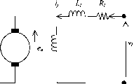 Rf Lf Ra La m-m---WYYY- (a) (b) FIGURE 27.2 (a) Separately excited dc motor circuit, (b) Series excited dc motor circuit. cOm, rad/sec cOm, rad/sec -ZNm TbNm  - Va increasi  Va increases Tr, Nm -COm (a) - COm, rad/sec (b) FIGURE 27.3 Torque-speed characteristics of (a) separately and (b) series-excited motors. in order to increase speed beyond the base speed. The armature voltage is now maintained at the rated value actively, by overriding the field control if required. Note that the range of field control is limited because of the magnetic nonlinearity of the field circuit and the problem of good commutation at weak field. Usually the top speed is limited to about three times the base speed. Note also that field weakening results in reduced torque production per ampere of armature current. Depending on the type of load, the armature current and speed change dictated by Eqs. (27.1)-(27.5). For the separately excited dc motor, assuming that the field excitation is held constant, the transfer characteristic between the shaft speed and the applied voltage to the armature can be expressed as indicated in the block diagram of Fig. 27.4. If we ignore the load torque T, the transfer characteristic is given V, isL, + RJUs + D) + KEKr the characteristic roots of which are given by (27.6) Va(s) Ea(s)
JtS + D (Om(s) Tl(s) FIGURE 27.4 excited motor. Transfer characteristic block diagram of a separately If we compare this with a standard second-order system, the undamped natural frequency and damping factor are given by (On =  1 D (27.8) (27.9) where s + - m = 0 (27.7) = mechanical time constant = KeKt in which = Kij: = Kj in SI units and = electrical time constant = -. The speed response of the motor around an operating speed to the apphcation of load torque on the shaft is given by 1+5T. ATr КЖт (l+5T,)(/5 + D)+ (27.10) 27.2.3 Converters for dc Drives Depending on application requirements, the power converter for a dc motor may be chosen from a number of topologies. For example, a half-controlled thyristor converter or a single-quadrant PWM switching converter may be adequate for a drive that does not require controlled deceleration with regenerative braking. On the other hand, a fuU four-quadrant thyristor or transistor converter for the armature circuit and a two-quadrant converter for the field circuit may be required for a high-performance drive with a wide speed range. The frequency at which the power converter is switched, e.g., 100 Fiz for a single-phase thyristor bridge converter supphed from a 50-Fiz ac source (or 300 Fiz for a three-phase thyristor bridge converter), 20 kFiz for a PWM MOSFET Fi-bridge converter, and so on, has a profound effect on the dynamics achievable with a motor drive. Low-power switching devices tend to have faster switching capability than high-power devices. This is convenient for low-power motors since these are normally required to be operated with high dynamic response and accuracy. 27.2.3.1 Thyristor Converter Drive Consider the dc drive of Fig. 27.5, for which the armature supply voltage to the motor is given by -cos a (27.11) Power Supply F С С VmaxSinCOt Ra La 4  where V is the peak value of the line-line ac supply voltage to the converter and a is the firing angle. The dc output voltage is controllable via the firing angle a, which in turn is controlled by the control voltage e as input to the firing control circuit (FCC). The FCC is synchronized with the mains ac supply and drives individual thyristors in the ac-dc converter according to the desired firing angle. Depending on the load and the speed of operation, the conduction of the current may become discontinuous as indicated in Fig. 27.6a. When this happens, the converter output voltage does not change with control voltage as proportionately as with continuous conduction. The motor speed now drops much more with load as indicated by Fig. 27.6b. The consequent loss of gain of the converter may have to be avoided or compensated if good control over speed is desired. The output voltage of the simple, two-pulse ac-dc converter of Fig. 27.5 is rich in ripples of frequency nf, where n is an even integer starting with 2 and / is the frequency of the ac supply. Such low-frequency ripple may derate the motor considerably. Converters with higher pulse number, such as the 6- or 12-pulse converter, deliver much smoother output voltage and may be desirable for more demanding applications. A high-performance dc drive for a rolhng miU drive may consist of such converter circuits connected for bi-directional operation of the drive, as indicated in Fig. 27.7. The interfacing of the firing control circuit to other motion-control loops, such as speed and position controUers, for the desired motion is also indicated. Two fully-controUed bridge ac-dc converter circuits are used back-to-back from the same ac supply. One is for forward and the other is for reverse driving of the motor. Since each is a two-quadrant converter, either may be used for regenerative braking of the motor. For this mode of operation, the braking converter, which operates in inversion mode, sinks the motor current aided by the back emf of the motor. The energy of the overhauhng motor now returns to the ac source. It may be noted that the braking converter may be used to maintain the braking current at the maximum aUowable level right down to zero speed. A complete acceleration-deceleration cycle of such a drive is indicated in Fig. 27.8. During braking, the firing angle is maintained at an appropriate value at aU times so that controUed and predictable deceleration takes place at aU times. - ai<90° 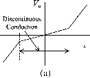 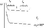 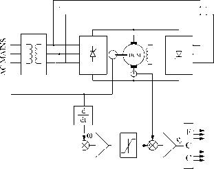 FIGURE 27.7 Bidirectional speed and position control system with a back-to-back (dual) thyristor converter. The innermost control loop indicated in Fig. 27.7 is for torque, which translates to an armature current loop for a dc drive. Speed- and position-control loops are usually designed as hierarchical control loops. Operation of each loop is sufficiently decoupled from the other so that each stage can be designed in isolation and operated with its special limiting features. 27.2.3.2 PWM Switching Converter Drive PWM switching converters have traditionally been referred to as choppers in many traction- and forklift-type drives. These are essentially PWM dc-dc converters operating from rectified dc or battery mains. These converters can also operate in one, two, or four quadrants, offering a few choices to meet application requirements. Servo drive systems normally use the full four-quadrant converter of Fig. 27.9, which allows bidirectional drive and regenerative braking capabilities. For forward driving, the transistors and T4 and diode D2 are used as a buck converter that supplies a variable voltage, v, to the armature given by = 3Vj (27.12) where У^ the dc supply voltage to the converter and 3 is the duty cycle of the transistor T. The duty cycle 3 is defined as the duration of the on time of the modulating (switching transistor) as a fraction of the switching period. The switching frequency is normally dictated by the application and the type of switching devices selected for the application. During regenerative braking in the forward direction, transistors t2 and diode D4 are used as a boost converter that regulates the braking current through the motor by automatically adjusting the duty cycle of t2. The energy of the overhauling motor now returns to the dc supply through diode D, aided by the motor back emf and the dc supply. Again, note that the braking converter, comprising t2 and , may be used to maintain the regenerative braking current at the maximum allowable level right down to zero speed. Figure 27.10 shows a typical acceleration-deceleration cycle of such a drive under the action of the control loops indicated in Fig. 27.9. 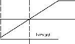 Forward Running Reverse Braking Acceleration Forward Runrung
Reverse Rmining FWD FWD I FWD 4<и IV I REV < . и <: с  DCM V-Q-
1 5 4 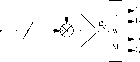 FIGURE 27.9 Bidirectional speed and position control system with a PWM transistor bridge drive. Four-quadrant PWM converter drives such as that in Fig. 27.10 are widely used for motion-control equipment in the automation industry. Because of significant development of power switching devices, switching frequencies of 10-20 kFiz are easily attainable. At such frequencies, virtually no derating of the motor is necessary. In order to satisfy the requirements of a drive apphcation, simpler versions of the drive circuits indicated in Figs. 27.7 and 27.9 may be used. For instance, for a unidirectional drive half of the converter circuits indicated earlier may be used. Further simphfication of the drive circuit is possible if regenerative braking is not required. FIGURE 27.11 dc drive. Structure of a closed-loop speed-control system with a 27.2.4 Drive System Integration A complete drive system has a torque controUer (armature current controUer for a dc drive) as its innermost loop, followed by a speed controller as indicated in Fig. 27.11. The inner current loop is often regulated with a proportional plus integral (PI) type controller of high gain. The rest of the inner loop consists of the converter, the motor armature, which is essentially an R-L circuit with armature back emf as disturbance, and the current sensor. The current sensor is typically an isolated circuit, such as a FiaU sensor or a direct-current transformer (DCCT). A weU-designed torque (armature current) loop behaves essentially as a first-order lag system. Together with the mechanical inertia load, this loop can be indicated as the middle Bode plot of Fig. 27.12, in which 1/T represents the current-controUed system bandwidth. (Note that the damping factor D and the load torque Tl indicated in Fig. 27.11 have been neglected in this description for simplicity.) The current loop is normally designed by analyzing the block diagram of Fig. 27.11, the converter, and Forward Forward Running Reverse Braking Acceleration Forward Running Forward Braking Reverse Acceleration 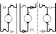 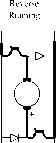 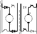
FIGURE 27.12 Typical current and speed control loop designs for the system of Fig. 27.11. the PI controller for the current loop using Bode analysis or other control-system design tools. The next step is usually the design of the speed controller. The 0-db intercept of 1 5(1 + Ts) is normally much too low. Again, if a PI controller is selected for the speed loop, its Bode plot is superimposed on the current controlled system as indicated in Fig. 27.12 to obtain the desired speed-control bandwidth. 27.2.5 Converter-DC Drive System Considerations Several operational factors need to be considered in applying a dc drive. Some of the important ones are as follows: 1. The armature current may be rich in harmonics. This is particularly true for thyristor converters. The feedback of these current ripples into the firing-control circuit may cause overloading of individual switches and tripping. Adequate filtering is necessary to avoid such problems. 2. Since the converter is switched at regular intervals while the current controller operates continuously, current overshoot may occur because of the delay in the firing-control circuit. The current controller gains must be hmited to limit this overshoot. 3. The switching frequency of the converter should be selected according to the desired motor-current ripple. supply-input current harmonics, and dynamic performance of the drive. 4. Ripple in the speed sensor output limits the performance of the speed controller. Analog tachogenerator output is particularly noisy and defines the upper limit of the speed control bandwidth. Digital speed sensors, such as encoders and resolvers, alleviate this limit significantly. 27.2.6 Further Reading 1. G. K. Dubey, Power Semiconductor Controlled Drives. Prentice Hall, 1989. 2. W. Leonard, Control of Electric Drives. Springer-Verlag, 1985. 3. V. Subrahmanyam, Electric Drives; Concepts and Applications. McGraw-Hill, 1994. 4. M. A. El-Sharkawi, Fundamentals of Electric Drives. Thompson Learning, 2000. 27.3 Induction Motor Drives M. F. Rahman 27.3.1 Introduction The ac induction motor is by far the most widely used motor in the industry. Traditionally, it has been used in constant and variable-speed drive apphcations that do not cater for fast dynamic processes. Because of the recent development of several new control technologies, such as vector and direct torque controls, this situation is changing rapidly. The underlying reason for this is the fact that the cage induction motor is much cheaper and more rugged than its competitor, the dc motor, in such applications. This section starts with induction motor drives that are based on the steady-state equivalent circuit of the motor, followed by vector-controlled drives that are based on its dynamic model. 27.3.2 Steady-State Representation The traditional methods of variable-speed drives are based on the equivalent circuit representation of the motor shown in Fig. 27.13. Rl Li 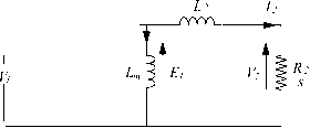 From this representation, the foUowing power relationships in terms of motor parameters and the rotor shp can be found Power in the rotor circuit, P2 = 3/ - = 3 .R2 s 3SR2EI rl(s(DL2f (27.13) Output power, Pq = P2- 3IJR2 = (1-S)P2 = CD,T (1 - s)co, where slip, 5 = P = number of pole pairs (27.U) (27.15) rad/s; N is the rotor speed in rev/min co = rotor speed in electrical rad/s = 2nfi rad/s (electrical), f being the supply frequency The developed torque T = T Nm Щ/Р (27.16) The shp frequency, 5/1, is the frequency of the rotor current, and the airgap voltage is given by £1 = щЬ = (27.17) where 1 is the stator flux hnkage due to the airgap flux. If the stator impedance is negligible compared to E, which is true when fl is near the rated frequency , ViEi= 2nfil, =--T coi rl SR2VI (sCDiL2r 3P sR2(2nfifli rl(scDiL2f (27.Щ (27.19) 27.3.3 Characteristics and Methods of Control The preceding analysis suggests several speed control methods. The foUowing are some of the widely used methods: 1. Stator voltage control 2. Slip power control 3. Variable-voltage, variable-frequency (V-/) control 4. Variable-current, variable-frequency (/-/) control These methods are sometimes caUed scalar controls to distinguish them from vector controls, which are described in Section 27.3.4. The torque-speed characteristics of the motor differ significantly under different types of control, as wiU be evident in the foUowing sections. 27.3.3.1 Stator Voltage Control In this method of control, back-to-back thyristors are used to supply the motor with variable ac voltage, as indicated in the converter circuit diagram of Fig. 27.14a. The analysis of Section 27.3.1 imphes that the developed torque varies inversely as the square of the input RMS voltage to the motor, as indicated in Fig. 27.14b. This makes such a drive suitable for fan- and impeUer-type loads for which torque demand rises faster with speed. For other types of loads, the suitable speed range is very hmited. Motors with high rotor resistance may offer an extended speed range. It should be noted that this type of drive with back-to-back thyristors with firing-angle control suffers from poor power and harmonic distortion factors when operated at low speed. If unbalanced operation is acceptable, the thyristors in one or two supply hnes to the motor may be bypassed. This offers the possibUity of dynamic braking or plugging, desirable in some applications. 27.3.3.2 Slip Power Control Variable-speed, three-phase, wound-rotor (or slip-ring) induction motor drives with slip power control may take several forms. In a passive scheme, the rotor power is rectified and dissipated in a hquid resistor or in a multitapped resistor that may be adjustable and forced cooled. In a more popular scheme, which is widely used in medium- to large-capacity pumping instaUations, the rectified rotor power is returned to the ac mains by a thyristor converter operating in naturally commutated inversion mode. This static Scherbius scheme is Load Г-СО 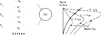 Torque, Nm indicated in Fig. 27.15. In this scheme, the rotor terminals are connected to a three-phase diode bridge that rectifies the rotor voltage. This rotor output is then inverted into mains fi-equency ac by a fiiUy controlled thyristor converter operating off the same mains as the motor stator. The converter in the rotor circuit handles only the rotor shp power, so that the cost of the power converter circuit can be much less than that of an equivalent inverter drive, albeit at the expense of the more expensive motor. The dc link current, smoothed by a reactor, may be regulated by controlhng the firing angle of the converter in order to maintain the developed torque at the level required by the load. The current controller (CC) and speed controller (SC) are also indicated in Fig. 27.15. The current controller output determines the converter firing angle a from the firing control circuit (FCC). From the equivalent circuit of Fig. 27.13 and ignoring the stator impedance, the RMS voltage per phase in the rotor circuit is given by V, CDr V, SCO, n CD, n CD, (27.20) where and are the angular frequencies of the voltages in the stator and rotor circuits, respectively, and n is the ratio of the equivalent stator to rotor turns. The dc-hnk voltage at the rectifier terminals of the rotor, v, is given by 3V6Vj, Assuming that the transformer interposed between the inverter output is and the ac supply has the same turn ratio n as the effective stator-to-rotor turns of the motor. 3V6 V, =---cosa (27.21) The negative sign arises because the thyristor converter develops negative dc voltage in the inverter mode of operation. The dc-link inductor is mainly to ensure continuous current through the converter so that the expression (27.21) holds for all conditions of operation. Combining the preceding three equations gives scD, = cosa so that 5 = -/7 cos a and the rotor speed cOq = -(1 - 5)0; = -шД1 + /7 cos a) rad/s. (27.22) Thus, the motor speed can be controlled by adjusting the firing angle a. By varying a between 180° and 90°, the speed of the motor can be varied from zero to full speed, respectively. For a motor with low rotor resistance and with the assumptions taken earlier, it can be shown that the developed torque of the motor is given by T = 3Pi 3P1J Nm (27.23) where is the dc link current. Thus, the inner torque control loop of a variable-speed drive using the Scherbius scheme MAINS 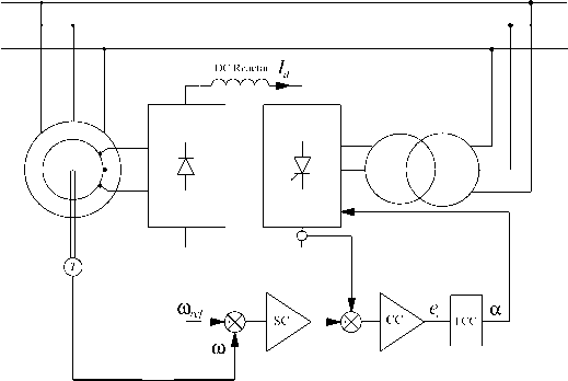 1 ... 64 65 66 67 68 69 70 ... 91 |
|||||||||||||||||||||||||||||||||||||||||||||||||||||||||||||||||||||||||||||||||
|
© 2026 AutoElektrix.ru
Частичное копирование материалов разрешено при условии активной ссылки |