 |
 |
 |
| Главная Журналы Популярное Audi - почему их так назвали? Как появилась марка Bmw? Откуда появился Lexus? Достижения и устремления Mercedes-Benz Первые модели Chevrolet Электромобиль Nissan Leaf |
Главная » Журналы » Metal oxide semiconductor 1 ... 65 66 67 68 69 70 71 ... 91 normally employs a dc-link current loop as the innermost torque loop. Figure 27.16 shows transient responses of the dc-link, rotor, and stator currents of such a drive when the motor is accelerated between two speeds. The drive is normally started with a short-time-rated liquid resistor, and the thyristor speed controller is started when the drive reaches a certain speed. By replacing the diode rectifier of Fig. 27.16 with another thyristor bridge, power can be made to flow to and from the rotor circuit, allowing the motor to operated at higher than synchronous speed. For very large drives, a cycloconverter may also be used in the rotor circuit with direct conversion of frequency between the ac supply and the rotor and driving the motor above and below synchronous speed. 27.3.3.3 Variable-Voltage, Variable-Frequency (V-f) Control 27,3,3,3,1 SPWM Inverter Drive When an induction motor is driven from an ideal ac voltage source, its normal operating speed is less than 5% below the synchronous speed, which is determined by the ac source frequency and the number of motor poles. With a sinusoidally modulated (SPWM) inverter, indicated in Fig. 27.17, the supply frequency to the motor can be easily adjusted for variable speed. Equation (27.18) imphes that if rated airgap flux is to be maintained at its rated value at all speeds, the supply voltage to the motor should be varied in proportion to the frequency f. The block diagram of Fig. 27.18a shows how the frequencyand the output voltage of the SPWM inverter are proportionately adjusted with the speed reference. The speed reference signal is normally passed through a filter that only aUows a gradual change in the AC . Mains ->Тз ->Т5  FIGURE 27.17 V-f drive with SPWM inverter. frequency f. This type of control is widely referred to as the V-f inverter drive. Control of the stator input voltage V as a function of the frequency f is readily arranged within the inverter by modulating the switches T-T. At low speed, however, where the input voltage V is low, most of the input voltage may drop across the stator impedance, leading to a reduction in airgap flux and loss of torque. Compensation for the stator resistance drop, as indicated in Fig. 27.18b, is often employed. Fiowever, if the motor becomes lightly loaded at low speed, the airgap flux may exceed the rated value, causing motor to overheat. Speed reference l + TfS reference reference -> 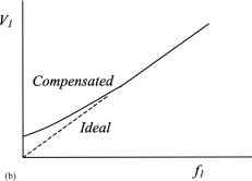 FIGURE 27.18 (a) Input reference filter and voltage and frequency reference generation for the V-f inverter drive, (b) Voltage compensation at low speed. From the equivalent circuit of Fig. 27.13 and neglecting rotor leakage inductance, the developed torque T and the rotor current /2 are given by (27.24) (27.25) where scd is the slip frequency, which is also the frequency of the voltages and currents in the rotor. Equation (27.24) implies that by limiting the shp 5, the rotor current can be limited, which in turn limits the developed torque [Eq. (27.25)]. Consequently, a slip-limited drive is also a torque-limited drive. Note that this true only at steady state. A speed-control system with such a slip limiter is shown in Fig. 27.19. In this scheme, the motor speed is sensed and added to a limited speed error (or hmited slip speed) to obtain the frequency (or speed reference for the V-f drive). Many applications of the V-f controller, however, are open-loop schemes, in which any demanded variation in V is passed through a ramp limiter (or filter) so that sudden changes in the slip speed cd. are precluded, thereby allowing Speed Controller FIGURE 27.19 Closed-loop speed controUer with an inner slip loop. the motor to follow the change in the supply frequency without exceeding the rotor current and torque limits. From the foregoing analyses, it is obvious that the V-f inverter drive essentially operates in all four quadrants, with rotor speed dropping shghtly with load, and developing full torque at the same slip speed at all speeds. This assumes that the stator input voltage is properly compensated so that the motor is operated with constant (or rated) airgap flux at all speed. The motor can be operated above the base speed by keeping the input voltage V constant while increasing the stator frequency above base frequency in order to run the motor at speeds higher than the base speed. The airgap flux and hence maximum developed torque now fall with speed, leading to constant power type characteristic. Figure 27.20 CO, rad/sec Sequence: a-c-b Base speed with rated Vj and base fi  Sequence: a-b-c Trated T,Nm FIGURE 27.20 Typical T-(d characteristics of V-f drive with input frequency fx and voltage V below and above base speed. depicts the T-co characteristics of such a vohage- and frequency-controUed drive for various operating frequencies. In this figure, the T-co characteristic for base speed has been drawn in fuU, indicating the maximum developed torque T and the rated torque. Below base speed, the Vi/f ratio is maintained to keep the airgap flux constant. Above base speed, Vl is kept constant, whUe f increases with speed, thus weakening the airgap flux. Forward driving in quadrant Ql takes place with an inverter output voltage sequence of a-b-c, whereas reverse driving in quadrant Q3 takes place with sequence a-c-b. Regenerative braking while forward driving takes place by adjusting the input frequency f in such a way that the motor operates in quadrant Q2 (quadrant Q4 for reverse braking) with the desired braking characteristic. Note that the characteristics in Fig. 27.20 are based on the steady-state equivalent circuit model of the motor. Such a drive suffers from poor torque response during transient operation because of time-dependent interactions between the stator and rotor fluxes. Figure 27.21 indicates the machine airgap flux during acceleration with V-f control obtained from a dynamic model. Clearly, the airgap flux does not remain constant during dynamic operation. 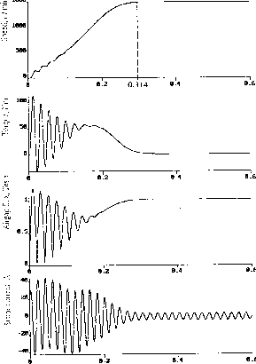 T, Sec. 27,3,3,3,2 Cycloconverter Drive For large-capacity induction motor drives, the variable-frequency supply at variable voltage is effectively obtained from a cycloconverter in which back-to-back thyristor converter pairs are used, one for each phase of the motor, as indicated in Fig. 27.22. Each thyristor block in this figure represents a fully controUed thyristor ac-dc converter. The maximum output frequency of such a converter can be as high as about 40% of the supply frequency. In view of the large number of thyristor switches required, cycloconverter drives are suitable for large-capacity but low-speed applications. 27.3.3.4 Variable-Current-Variable-Frequency (/-/) Control In this scheme, medium- to large-capacity induction motors are driven from a variable but stiff current supply that may be obtained from a thyristor converter and a dc link inductor as indicated in Fig. 27.23. The frequency of the current supply to the motor is adjusted by a thyristor converter with auxUiary diodes and capacitors. The diodes in each inverter leg and the capacitors across them are needed for turning off the thyristors when current is to be commutated from one to the next in sequence. The motor current waveforms are normally six-step, or quasi square, as indicated in Fig. 27.24. The switching states of the inverter thyristors are also indicated in this figure. The motor voltage waveforms are determined by the load. These waveforms are more nearly sinusoidal than the current waveforms. The thyristor converter supplying the quasi-square current waveforms to the motor has firing angle control, in order to regulate the dc-hnk current to the inverter. The dynamics of the dc-hnk current control is such that this current may be considered to be constant during the time the inverter switches commutate the dc-link current from one switch to the next. Such a current-source drive offers four-quadrant operation, with independent control of the dc-link current and output frequency. One drawback is that the motor voltage waveforms have voltage spikes due to commutation. From the analysis of Section 27.3.2, if the higher order harmonics of the current waveforms in Fig. 27.24 are neglected, and it is assumed that the motor voltage and current waveforms are taken to be sinusoidal, the magnetizing current in Fig. 27.13 can be kept constant (for constant-airgap flux operation) if the RMS value of the stator supply current II is defined according to Eq. (27.26). This relationship is also shown in graphical form in Fig. 27.25. L = I Rl + jlnfisLf Rl2nfi(L2Lj nl/2 = constant (27.26) The control scheme for variable-speed operation with a current source drive is indicated the block diagram of Fig. 27.26. The speed reference defines the stator current reference transformer bank и В с  FIGURE 27.22 V-f drive with cycloconverter drive. according to Eq. (27.26) and the frequency reference is obtained by adding the rotor frequency to the actual speed of the motor. The inverter drive may consist of the thyristor current source and inverter of Fig. 27.23 or the diode-rectifier-supphed SPWM transistor inverter of Fig. 27.17 with independent current regulators, one for each phase. The dynamic performance of such current-controlled induction motor drives is not very satisfactory, just as for the voltage source inverters. Furthermore, the current-source rectifier
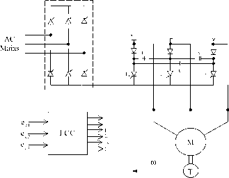 inverter drive cannot normally be operated open-loop, like the V-f inverter drive. For high dynamic performance, vector-controlled drives are becoming popular. 27.3.4 Vector Controls The foregoing scalar control methods are only suitable for adjustable-speed applications in which the load speed or position is not controlled as in a servo system. The vector control technique allows a squirrel-cage induction motor to be driven with high dynamic performance, comparable to that of a dc motor. For this, the controller needs to know the rotor speed (in the indirect method) or the airgap flux vector accurately, using sensors. The latter method is not practical because of the requirement of attaching airgap flux sensors. + Id- -I, - Тб j T, FIGURE 27.23 Dc-link current-source thyristor inverter drive. Stator current (A) 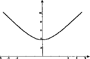 -2-1012 Rotor frequency (Hz) FIGURE 27.25 Stator current vs rotor (slip) frequency for constant-airgap flux operation. 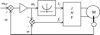 FIGURE 27.26 Variable-current, variable-frequency inverter drive scheme. The indirect method, which is being widely accepted in recent years, requires the controUer to be matched with the motor being driven. This is because the controUer needs also to know some rotor parameter(s), which may vary according to the conditions of operation, continuously. 27.3.4.1 Basic Principles The methods of vector control are based on the dynamic equivalent circuit of the induction motor. There are at least three fluxes (rotor, airgap, and stator) and three currents or mmfs (stator, rotor, and magnetizing) in an induction motor. For high dynamic response, interactions among current, fluxes, and speed must be taken into account in determining appropriate control strategies. These interactions are understood only via the dynamic model of the motor. AU fluxes rotate at synchronous speed. The three-phase currents create mmfs (stator and rotor) that also rotate at synchronous speed. Vector control aligns axes of an mmf and a flux orthogonally at aU times. It is easier to align the stator current mmf orthogonally to the rotor flux. Any three-phase sinusoidal set of quantities in the stator can be transformed to an orthogonal reference frame by /о cosO cos( sm и sm\ и -- sini в- fas fbs fcs (27.27) where в is the angle of the orthogonal set with respect to any arbitrary reference. If the axes are stationary and the a axis is aligned with the stator a axis, then в = 0 at aU times. Thus Jos. V3 V3 fas fbs .fcs. (27.28) If the orthogonal set of reference rotates at the synchronous speed 1, its angular position at any instant is given by CO, f + 0n (27.29) The orthogonal set is then referred to as d-q-0 axes. The three-phase rotor variables, transformed to the synchronously rotating frame, are fdr f,r fo C0s(C0-C0)t COSco-co)t- COSTCO-co)t- sm{(D-(jo)t smi (cOg-cojt--j smi (ш^-cojt-- far fbr Ifcr] (27.30) It should be noted that the difference - is the relative speed between the synchronously rotating reference frame and the frame attached to the rotor. This difference is the also slip frequency, cd which is frequency of the rotor variables. By applying these transformations, voltage equations of the motor in the synchronously rotating frame reduce to The stator flux linkage equations are \s = Us\s + m(V + V) = 5 V + V (27.32) ds = Ushs + Lm{4s + hr) = Lsids + LJdr (27.33) (27.34) pLm ((Oe-r)Lm Rr РЦ i0J,-(D,)L, -(ш,-ш,) pL -{оэ,-со,)Ц Rr+pL, The rotor flux linkages are given by dr = Urhr + m(4 + 4r) = Lridr + LJds (27.36) (27.31) where the speed of the reference frame, ш^, is equal to co and Subscripts / and m stand for leakage and magnetizing, respectively, and p represents the differential operator d/dt. The equivalent circuits of the motor in this reference frame are indicated in Figs. 27.27a and 27.27b. n COeXds Lis r r Llr (C0e-C0r)Xdr R, - Iqs Iqr JTYYV- > I < rYYYV (a) ids idr JTYYV- > I < ((Oe-(Or)Xqr FIGURE 27.27 Motor dynamic equivalent circuits in the synchronously rotating (a) q- and (b) J-axes. - \l (qr + dr) The airgap flux linkages are given by md = Lm(.4s + 4r) m - \l imqs + mds) The torque developed by the motor is given by 3P From Eq. (27.39), the rotor voltage equations are i;, = 0 = + (CO, - CD,)LJds + {Rr + (27.37) (27.38) (27.39) (27.40) (27.41) + (со, - (D,)L,idr Vdr = 0 = L (CO, - CD,)LJ, + (R, + L,) (27.42) Using (27.35) and (27.36), (27.43) + Я V + - = 0 (27.44) dr + R,idr + (Ш, - CD,)X = 0 (27.45) Also from (27.35) and (27.36), -I2 -hi- (27.46) (27.47) The rotor currents i and i can be ehminated from (27.44) and (27.45) by using (27.46) and (27.47). Thus qr (27.48) - R,i, + (CO, - co,)Ad, = 0 (27.49) is reduced in order to weaken the rotor flux so that the motor may be driven with a constant-power-hke characteristic. Based on how the rotor flux is detected and regulated, two methods of control are available. One is the more popular indirect-rotor flux-oriented control (IFOC) method, and the other is the direct vector control method; both are described hereafter. A condition for elimination of transients in rotor flux and the coupling between the two axes is to have The rotor flux should also remain constant so that From (27.50) and (27.51), L R . + 1 -L i (27.50) (27.51) (27.52) (27.53) Substituting the expressions for i and i into (27.35) and (27.36), (27.55) Substituting and from (27.54) and (27.55) into the torque equation of (27.41) ~ ~ Tdrqs ~ qrds) - ~ ~r\s 2 и (27.56) It is clear from (27.53) that the rotor flux is determined by ij, subject a time delay that is the rotor time constant (LJR). Current i, according to Eq. (27.56), controls the developed torque T without delay. Currents i and i are orthogonal to each other and are called the flux and torque-producing currents, respectively. This correspondence between flux and torque-producing currents is subject to maintaining the conditions in (27.50) and (27.51). Normally, i would remain fixed for operation up to the base speed. Thereafter, it 27.3.4.2 Indirect-Rotor Flux-Oriented (IFOC) Vector Control In the indirect scheme, the relationship between slip frequency and given by (27.52) is used to relate the compensated speed error - to i. The i, in turn, is used to develop to the demanded torque according to (27.56). The rotor flux is maintained at the base value for operation below speed, and it may be reduced to a lower value for field weakening above base speed. The orthogonal relationship between the torque-producing stator current i and the flux-producing stator current i is maintained at all times by generating the stator current references in the synchronously rotating dq reference frame using sine and cosine functions of angle 9i. This angle is obtained as indicated in Fig. 27.28. The compensated speed error produces the current reference according to (27.56). i* also gives the slip speed сЭф according to (27.53). The slip speed coj is added to the rotor speed Ш, to obtain the stator frequency ш^. This frequency is integrated with respect to time to produce the required angle в I of the stator mmf relative to the rotor flux vector. This angle is used to transform the stator currents to the dq reference frame. Two independent current controUers are used to regulate the and currents to their reference values. The compensated and errors are then inverse transformed into the stator a-b-c reference frame for obtaining switching signals for the inverter via PWM or hysteresis comparators. It is clear that this scheme uses a feed-forward scheme, or a machine model, in which the current reference for i is also determined by the rotor time constant T. This also indicated in Fig. 27.28. The rotor time constant cannot be expected to remain constant for aU conditions of operation. Its considerable variation with operating conditions means that the slip speed сОф which directly affects the developed torque and the rotor flux vector position, may vary widely. Many rotor time-constant identification schemes have been developed in recent years to overcome the problem. The mandatory requirement for a rotor-speed sensor is also a significant drawback, because its presence reduces the rehabUity of the IFOC drive. Consequently, sensorless schemes of identifying the rotor flux position have also drawn considerable interest in recent years. Figure 27.29 shows the transient response of an induction motor that was for the results of Fig. 27.21 under the IFOC Speed Controller + A.  (Osl (01 7\ + Current Controllers qs + 60, ( FIGURE 27.28 Indirect-rotor flux-oriented vector control scheme. 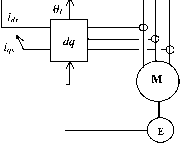 drive scheme of Fig. 27.28. In this case, the drive accelerates a large inertia load from standstill to the base speed of 1500rev/min. It is clear that the overcurrent transients of Fig. 27.21 are eliminated, while the motor accelerates under constant torque (imphed by the constant rate at which the speed increases) and settles at the final speed with little over-or undershoot in speed. Obviously, rotor and airgap fluxes remain constant at all times. 27.3.4.3 Direct Vector Control with Airgap Flux Sensing In the direct scheme, use is made of the airgap flux hnkages in the stator d- and -axes, which are then compensated for the respective leakage fluxes in order to determine the rotor flux linkages in the stator reference frame. The airgap flux linkages are measured by instaUing quadrature flux sensors in the airgap, as indicated in Fig. 27.30. By returning to Eqs. (27.32)-(27.40) in the stator reference frame and using some simplifications, it can be shown that 1500rev/mir n s 12 J -s qr ~ J qm Hr-qs dr = Y~dm ~ Цг5 (27.57) (27.58) 3.4 Amp 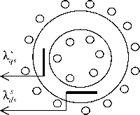 where the superscript 5 stands for the stator reference frame. Since the rotor flux rotates at synchronous speed with respect to the stator reference frame, the angle 9i used for the coordinate transformations in Fig. 27.27 can be obtained from cos = where (27.59) (27.60) popular in recent years in the form of permanent-magnet brushless dc and ac synchronous motor drives in servo-type applications. There are certain features of three-phase synchronous motors that have allowed them, especially the lower capacity motors, to be controUed with high dynamic performance using cheaper control hardware than is required for the induction motor of simUar capacity. Since the average speed of the synchronous motor is precisely related to the supply frequency, which can be precisely controUed, multi-motor drives with a fixed speed ratio among them are also good candidates for synchronous motor drives. This section begins with the performance of the variable-speed nonsalient-pole and sahent-pole synchronous motor drive using the steady-state equivalent circuit foUowed by dynamics of the vector-controUed synchronous motor drive. The control of torque via i and rotor flux via i subject to satisfying conditions (27.50) and (27.51); remain as indicated in Fig. 27.28, according to the basic principle of vector control. The requirement of airgap flux sensors is rather restrictive. Such fittings also reduce reliability. Even though this method of control offers better low-speed performance than the IFOC, this restriction has practically precluded the adoption of this scheme. In an alternative method, the d- and -axis stator flux linkages of the motor may be computed from integrating the stator input voltages. 27.3.5 Further Reading 1. B. K. Bose, Power Electronics and ac Drives. Prentice Hall, 1987. 2. J. M. D. Murphy and G. G. TurnbuU, Power Electronic Control of ac Motors. Pergamon Press, 1988. 3. D. W. Novotny and T. A. Lipo, Vector Control and Dynamics of Drives. Oxford Science Publications, 1996. 4. P. Vas, Electrical Machines and Drives: A Space Vector Theory Approach. Clarendon Press, 1992. 5. G. K. Dubey, Power Semiconductor Controlled Drives. Prentice Hall, 1989. 27.4.2 Steady-State Equivalent-Circuit Representation of the Motor Some of the operating characteristics of variable-frequency voltage- and current-source-driven synchronous motors can be readily obtained from their steady-state equivalent representation, as was the case with the scalar controls of induction motor drives. Assuming balanced, sinusoidal distribution of stator and rotor MMFs and an uniform airgap (nonsalient-pole motor), the per-phase equivalent circuit of Fig. 27.31 represents the motor at a constant speed. The representation in the figure is in terms of the RMS voltage V applied to the motor phase winding, which consists of the phase resistance R, synchronous reactance (in Q/phase), and the per-phase induced voltage E. The back emf Ef develops in the stator phase winding as a result of rotor excitation supplied from an external dc source via slip rings or by permanent magnets in the rotor. The phasor E has an arbitrary phase angle д with respect to the input voltage V. This is the load angle of the motor. Unlike the induction motor, a synchronous motor may derive part or aU of its excitation from the rotor via rotor excitation. For smaU synchronous motors that are used in 27.4 Synchronous Motor Drives M. F. Rahman 27.4.1 Introduction Variable-speed synchronous motors have been widely used in very large capacity (>MW) pumping and centrifuge type apphcations using naturally commutated current-source thyristor converters. At the low-power end, the current-source SPWM inverter-driven synchronous motors have become very VZO° jXs=JcoLs I -mm->-   EfZS° brushless dc and ac servo applications, this excitation is derived from permanent magnets in the rotor. This is readily and economically obtained with modern permanent magnets, thus dispensing with the shp-ring-brush assembly. The fR losses in the rotor windings with external excitation are also ehminated. These magnets also allow considerable reduction in space requirement for the rotor excitation. For large synchronous motors, this excitation is supplied more economically from an external dc source via slip rings or via an exciter. The phasor diagrams of Fig. 27.32 may be used to analyze characteristics of the nonsalient-pole synchronous motor drive. Since the rotor magnetic field may be such that the motor may develop a back emf that is smaller or larger than the ac supply voltage to the stator windings, the motor may accordingly be under- or overexcited, respectively. The overexcited motor will normally operate at a leading power factor, as is the case in Fig. 27.32b. This is desirable in high-power applications. In the phasor diagrams of Fig. 27.32c, the stator current / has been resolved into two components 1 and which are current phasors responsible for developing MMFs in the rotor d- and -axes. These representations are in the stator reference frame, and hence are sinusoidal quantities at the frequency of the stator supply. If the voltage drop across the stator resistance is neglected, which may be acceptable when the stator frequency is near the base frequency or higher, the developed torque T of the motor can be found from the phasor relationships of Fig. 27.32. Thus, 3 £У . 3P EV . 3PiC У T =--sm 0 =--sm о =-- - sm о Nm co CO coL Ц CO for the nonsahent-pole motor (also for the sine-wave PM ac motor with rotor magnets at the surface of the rotor) and 3P T = - = 3P sm d H--I -I sm 2d cold Кф V - smd+-  Nm sin 2 (27.62) (27.61) for the salient-pole motor (also for the interior-magnet motor in which the rotor magnets are buried inside the rotor). Here the flux constant of the motor, Кф, is the ratio of the RMS value of the phase voltage Ef induced in the stator due to rotor excitation only and speed. Note that for a given rotor excitation, the ratio Кф = E/cd remains constant at all speeds. 27.4.3 Performance with Voltage Source Drive Equations (27.61) and (27.62) imply that if the motor is driven from a voltage-source supply and if the input voltage to frequency ratio, is kept constant, the motor will develop the same maximum torque at all speeds. For the nonsalient-pole motor, this maximum torque will occur for a load angle д = 90°. For the salient-pole motor, this will occur for a load angle which is also influenced by the relative values of and L. At low speed, where the supply voltage V is small, the voltage drop in the stator resistance may become significant compared to E. This may lead to a significant drop in the maximum available torque, as given by the torque Eqs. (27.63) and (27.64), which are derived from the phasor diagrams of 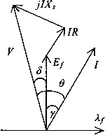 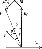 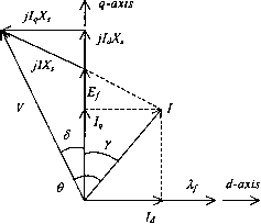 1 ... 65 66 67 68 69 70 71 ... 91 |
|||||||||||||||||||||||||||||||||||||||||||||||||||||||||||||||||||||||
|
© 2026 AutoElektrix.ru
Частичное копирование материалов разрешено при условии активной ссылки |