inverse d-q

transformation

INVERTER

d

transforaiation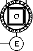

FIGURE 27.52 Block diagram of current-controlled drive.

In the second scheme, the motor currents are first transformed into the rotor (i-reference frame using continuous rotor-position feedback, and the measured rotor d- and -axis currents are then regulated in the rotor reference frame, as indicated in Fig. 27.52. The main advantage of regulating the stator currents in the rotor reference frame, compared to the stator reference frame as in the first scheme, is that current references now vary more slowly and hence suffer from lower tracking error. At constant speed, the stator current references are in fact dc quantities as opposed to ac quantities, and hence the inevitable tracking errors of the former scheme are easily removed by a integral type controUer. The other advantage is that the current references may now include feed-forward decouphng so as to remove the cross couphng of the d- and -axis variables as shown in the motor representation of Fig. 27.44. The latter scheme is currently preferred, since it aUows more direct control of the currents in the rotor reference frame.

It should be noted that continuous transformations to and from rotor dq-axes are required; hence the rotor-position sensor is a mandatory requirement. Rotor-position sensors of 10-to 12-bit accuracy are normally required. This is generally viewed as a weakness for this type of drive.

The general torque relationship of a sine-wave motor supplied from a current-source SPWM inverter is given by Eq. (27.69), which is rewritten here

Т = 1Р(Ф^(1,-1)щ)

(27.74)

Precise control of the developed torque control requires that both and be actively controUed in order to regulate it to the level determined by the error of the speed controller. For the surface-magnet synchronous motor, the large effective airgap means that L, so that should be maintained at zero level. This implies that the current reference in Fig. 27.52 should be kept zero. For the interior magnet motor, > so that and have to be controUed simultaneously to develop the desired torque. A few modes of operation are possible.

27.5.3.2 Operating Modes

27,5,3,2,1 Operation with Maximum Torque per Ampere (MTPA) Characteristic In this mode of control, the developed torque T per ampere of stator current is the highest for a given rotor excitation. The combination of and that develops the maximum torque per ampere of stator current is indicated in Fig. 27.53. The reference signal for the inner

Maximum torque -per-ampere trajectory

iq,A

2200 rpm Ф В

2400 rpm

TOOOrpm

Current limit

С

1500 фт

О

и, А

torque loop normally determines the reference; the reference is given by

2(Lq-Ld) .4(Lq-Ld)

.2 + 1

(27.75)

It should be noted that with = 0, this mode of operation is achieved for the surface magnet motor.

27.5.3.2.2 Operation with Voltage and Current Limits The

maximum current limit of the motor/inverter, Ismax is normally imposed by setting appropriate hmits on and such that

il + i\ < 4

(27.76)

Equation (27.75) defines a circle around the origin of the i-iq plane.

The available dc-link voltage to the inverter places an upper limit of the motor phase voltage, V, given by

V = Vj + Vj < vl,

nLf + {Ldh + Xf)<

(27.77) (27.78)

where the stator voltages and are expressed in the rotor reference frame, as in Eq. (27.68). Equation (27.78) is obtained from the voltage equation of (27.68) when the phase resistance R is neglected. Equation (27.78) defines elhptical trajectories that contract as speed increases. All three modes of operation are included in Fig. 27.53.

27.5.3.2.3 Operation with Field Weakening This mode of operation is normally required for operating the motor above the base speed. A constant-power characteristic is normally desired over the full field-weakening range. For a given rotor excitation of and developed power of P, the developed torque T and the net rotor flux linkage required for constant-power operation can be determined. From this, the limiting values for and i, which further constrain the allowable i-i trajectory as is also indicated in Fig. 27.53, can be determined.

The operating modes described in the preceding section are normally included in a trajectory controller that generates the references for and continuously, as indicated in Fig. 27.54.

Trajectory Generator

27.5.4 Further Reading

1. T. J. E. MiUer, Brushless Permanent Magnet and Reluctance Motor Drives. Oxford Science Publications, 1989.

2. Performance and Design of Permanent Magnet AC Motor Drives , Tutorial course, IEEE IAS Society, 1989.

3. R. M. Crowder, Electric Drives and Their Controls. Oxford Science Pubhcations, 1995.

27.6 Permanent-Magnet Brushless dc (BLDC) Motor Drives

D. Patterson

27.6.1 Machine Background

Anyone studying electric machines would be aware that the classical synchronous machine offers the possibihty of the very highest efficiencies. These machines have the power-carrying conductors in the stationary part; therefore, there is no need to transfer high power through a brush system. The field is provided on the rotating part either by an electromagnet, which does require some very low-power brushes, or at best by a permanent magnet with no power requirements at all.

This is clearly better than the traditional dc machine with high-power brushes dand rotating conductors, which also provide a very poor path for heat to get away from the rotor under overload conditions. You might well then ask, why did we use so many of them? It was of course because the dc machine offered the ability to control the speed fully and easily, which the synchronous machine, when running from the mains at a fixed frequency, definitely could not do. Thus, for example, all electric trains and trams built up to the 1980s, many of them still in service, use brushed dc motors.

The induction machine, the workhorse of industry, is quite efficient, but because of the need to carry magnetizing current in the stator as well as load current, and the existence of slip, it cannot be as good as the synchronous machine. It also innately has a very hmited speed range.

All this changed with the advent of inexpensive, reliable power electronics. Quite suddenly power-electronics engineers had the ability to vary both the frequency and the amplitude of an ac supply and thus to provide the holy grail of variable-speed ac motors. This was first apphed to induction machines, with the simplest form of open-loop control. The complexity of control for synchronous machines added substantially to the cost and was not so appeahng. Today the thought of putting a digital signal processor (DSP) or a microcontroller in a small motor controller is no longer as daunting as it was 10 years ago, so the distinction between the complexity of a controller for induction machines and synchronous machines has almost disappeared.

Although power electronics radically changed our attitudes towards electric machine design and operation, there was a

second very important development that arrived on the scene at almost the same time; the appearance of very powerful rare-earth permanent-magnet materials.

The first rare-earth magnet material was samarium-cobalt, used in very special applications such as space and defense, but it was then, and stiU is, very expensive. Neodymium-iron-boron (NdFeB) came next with even higher energy product. Energy product is a measure used to quantify the effectiveness of magnets. NdFeB began expensively, but has continued to drop in price at a spectacular rate and recently became cheaper than ferrites in term of doUars per unit of energy product. Thus, aU the machines discussed here are permanent magnet (PM) machines, in general using NdFeB magnets.

27.6.1.1 Clarifying Torque vs Speed Control

As is weU understood, given a fixed magnetic flux level, the magnitude of the current in a motor determines the magnitude of the torque out of the machine. In a general apphcation if a torque is set, the speed is determined by the load. This is what happens when driving an automobile. The throttle or accelerator varies the torque. The speed can be very slow or very high for the same foot position, depending on the road conditions and vehicle motion history, even if the vehicle is in the same gear. This principle of torque control rather than speed control is fundamental to the operation of electric machines. When speed control is required in PM BLDCMs, it is usual to implement torque control, with an extra outside control loop, like a cruise control in an automobile, to use the torque control to deliver speed control. So from here on the discussion will describe torque control for the variable speed motor.

27.6.1.2 Permanent-Magnet ac Machines

There are two quite different types of permanent-magnet ac machines, actually looking very similar in their physical realization but dramatically different in their electrical characteristics and in the way in which they are controUed.

27,6,1,2,1 Permanent-Magnet Synchronous Machines These are simple extensions of the classical synchronous machine, where aU of the voltages and currents are designed to be sinusoidal functions of time, as they are in the synchronous machine when used as a supply generator. These machines are known as permanent-magnet synchronous machines (PMSMs) or brushless ac machines and are discussed elsewhere in this book. Although the application of sinusoidal waveforms everywhere is comforting to many and does result in less acoustic noise, fewer stray losses, etc., there is in general a requirement to know the exact rotor angular position at every instant of time, with an accuracy on the order of 1°. This knowledge is then used to shape the current waveforms to be sure that they are in phase with the back emf of the windings. Although much research is going on to run these machines without position sensors, the reality in the

workplace today is that a relatively expensive shaft-position encoder is needed with a PMSM in order to control it electronically.

27,6,1,2,2 Permanent-Magnet Brushless dc Machines A

very much simpler possibUity has emerged, which also gives the benefits of smooth torque and rapid controUabUity. This results in smaUer minimum machine size, yielding maximum machine power density.

For this variant, the current waveforms and the back emf waveforms are trapezoidal rather than sinusoidal. In this case the machine is known as a permanent-magnet brushless dc machine (PMBDCM), with waveforms as shown in Fig. 27.55.

27.6.1.3 Brief Tutorial on Electric Machine Operation

The operation of electric machines can be explained in a variety of ways. Two possible and different methods are as foUows:

1. Using an understanding of the interaction of magnetic fields and the tendency of magnetic fields to ahgn. This tendency to align is what provides the force that makes a compass needle swing around untU it aligns with the earths magnetic field.

2. Using the physical principle that a current-carrying conductor in a magnetic field has a force exerted on it. This force is commonly known as the Lorentz force.

The difference between the two explanations is that the first method gives better physical pictures. Fiowever, when one gets a little more serious, wanting to put in numbers, the force equations, although not greatly more difficult, are a little more challenging as they involve vector cross products.

With the second method, once the principle is accepted, there is a particularly simple scalar version of the force

angle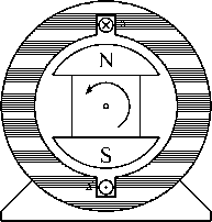

FIGURE 27.56 A simple motor with a single coil in the stator and a permanent-magnet rotor.

FIGURE 27.57 A computer-generated magnetic field for current in the windings and a stator; the stator is made of electrical steel.

equation that very rapidly and simply gives numeric answers. The directions of the force, current, and motion are all orthogonal, i.e., at right angles, and a formal exposition would again use a vector cross product. The familiar force equation, F = BLI, can be used, where F is the force in newtons, В is the flux density in teslas, L is the length of the conductor in meters, and / is the current in amperes.

Consider the simple machine of Fig. 27.56. The rotor is a magnet with a north and a south pole, and there is a coil of wire in the slots in the stator. Current is shown going into the conductor called a at the top of the stator and coming out of the conductor called a at the bottom. To simulate a real machine more closely, one should imagine putting a one-turn coil of wire into the slot, with a connection made at the back of the machine to connect the top wire to the bottom, so that when applying a positive voltage is applied to the top wire and a negative voltage to the end of the coil (the bottom wire), current will flow in at the top and out at the bottom as discussed previously.

27.6.1.3.1 Method 1 If the current is flows into the top and comes out of the bottom as marked, then according to the right-hand rule magnetic flux will be forced to go through the center of the coil from right to left, creating a north pole on the left. The flux will then double back through the iron frame of the motor to arrive back at the south pole on the right.

Figure 27.57 shows a computer-generated magnetic-field plot. This was produced using finite element analysis and modeling the stator as electrical steel, the volume in the center as air, and injecting current into the coil. If the permanent-magnet rotor is then put inside the stator of Fig. 27.57, the rotor will align by rotating 270° counterclockwise.

27.6.1.3.2 Method 2 In this case, looking at Fig. 27.58, the conductor a will be immersed in a quite dense field produced by the magnets, with the flux lines going up the page in the rotor, across the airgap into the steel of the stator, and heading

down the stator to jump back across the lower airgap to return to the south pole. If a current is directed into the upper conductor and out of the bottom as before, it will produce forces. Applying the direction rules associated with the Lorentz force, the force on the conductor will be to the right at the top and to the left at the bottom. Invoking Newton s third law, which states that action and reaction are equal and opposite, it is clear that if the wire is fixed, as it is, then there will be a force on the rotor to the left at the top and to the right at the bottom; thus, the rotor will move counterclockwise as before.

27.6.2 Electronic Commutation

If the rotor of Fig. 27.58 moves, then to keep it rotating in the same direction, sooner or later the current in the conductors must be reversed. The time at which that needs to be done is when the rotor has moved to an almost aligned position. Thus, it is not really a matter of time, but rather of rotor position. Since the rotor is a permanent magnet, it is a very simple matter to determine at least where the physical pole edges are, using simple, reliable, and inexpensive Hall-effect (HE) sensors. These are small semiconductor devices that respond to magnetic flux density. (There are many ways to sense the

Force on conductor a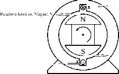

Reaction force on Magnet S

Force on conductor aL

FIGURE 27.58

machine.

position of the rotor; however, the remainder of this exposition wiU stay with the HE sensor for simphcity.)

A very simple motor, relying on the inertia of the rotor for continuous rotation, could have a control circuit which sensed when the rotor magnet was horizontal and then reversed the current in aa of Fig. 27.58.

The traditional Fi bridge switching circuit shown in Fig. 27.59 does that very effectively. Switch drive logic must ensure that either SI and S4 are on or S2 and S3 are on, and never SI and S2 simultaneously, or S3 and S4 simultaneously. This simultaneous operation would provide a short circuit. When this happens because of errors in the switch-drive signal it is caUed shoot-through. There are generally important parts of the switch drive signal logic, discussed later, that try to make this impossible in normal operation.

In real motors the permanent-magnet rotor field does not change instantaneously from north to south as the rotor rotates, so there would be reasonably large angles over which torque could not be effectively produced. Also, more coils are put in so that the space of the machine frame is used more efficiently.

The use of three phases, as in Fig. 27.60, is very common. There are many things that balance naturally in a three-phase system, and it is the simplest system with which it is possible

to develop constant and unidirectional torque at aU times and positions.

A very common method has developed, known as six-step switching . In this system three phases are used, and connected in a star shape. There is a space between each of the magnet poles on the rotor and two phases are activated at any one time, the third resting as the space between the magnet poles passes over it.

Although the motor in Fig. 27.60 looks just like a three-phase synchronous machine, its operation is rather different. As just stated, the windings are invariably star-connected, as shown in Fig. 27.61.

27.6.2.1 Six-Step Switching Explained

Consider the coil aa as shown in Fig. 27.60 and also diagrammatically in Fig. 27.61. Current driven into the a terminal, coming out of the terminal, wiU produce, as discussed before, flux from left to right, as shown here.

Obviously, if the current direction in aa is reversed, the flux wiU be: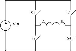

FIGURE 27.59 An H bridge circuit that can reverse the current through aa as drawn with mechanical switches.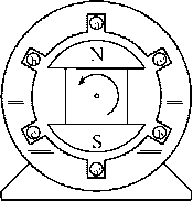

Similarly if current is driven into b and out of b flux wiU result:

And if it is reversed.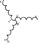

Finally, if current is driven into с and out of c flux will result:

the fourth of the cases just shown occur at the same time. They add to produce a resultant.

And if it is reversed.

The permanent magnet rotor would tend to align with the flux arrow shown in each of the states just shown, as discussed in Section 27.6.1.3.1.

Now if the motor is wired in a star as shown in Fig. 27.61 and a steady current is driven into a and out of b, the first and

and the rotor will tend to align with this resultant.

The Hall-effect sensors are positioned so that just as the rotor gets to this point, another arrangement of the windings is energized, and the rotor is pulled around another 60°. The rotor never quite achieves its desired position!

If a controller has input power from positive and negative of a dc supply and outputs to the terminals a, b, and с only, then the sequence of connections shown in Table 27.2 below will produce the resultant flux directions as shown, providing continuous rotation.

The switching of Table 27.2 is simply achieved by a variant of the H bridge, as shown in Fig. 27.62. This process of switching current into different windings is called commutation and is the equivalent of the sliding brush contacts in a traditional brushed dc machine.

TABLE 27.2 Sequence of connections that results in counterclockwise continuous rotation of the rotor of the PM BLDC motor of Fig. 27.60

When Rotor is at This Position, Connections are Made as at Right

Terminal a

Terminal b Terminal с

Flux Directions

Current in

Zero

Current out Zero

Current out Current in

Current out Zero

Current in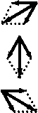

Current out Current in Zero

Zero

Current in Current out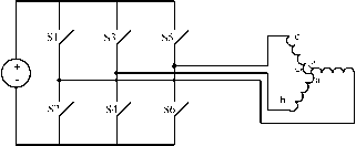

FIGURE 27.62 The switching circuit used for commutation of a PM BLDC motor.

27.6.3 Current/Torque Control

The preceding discussion has been about current in the windings rather than vohage across them. In very simple, very smaU brushless dc machines, such as the one in the muffin fan in a computer power supply, voltages are connected directly to the windings. For these smaU motors the resistance of the windings is relatively high, and this helps limit the actual current that flows and swamps inductive effects.

There is an extra difficulty that must be addressed with high-performance, high-efficiency, weU-made machines and it adds another layer to the control of the motor. Such machines can easily be designed with very low-resistance windings. It is not uncommon to have windings for a 200-V machine at the 20-kW level with winding resistances of less than 0.1 Q.

When starting, or at a low speed, the current in a winding is limited only by the very low resistance, and for the machine in this example, by Ohms law, I = E/R would result in more than 2000 A!

The most common requirement is for a steady current in the windings, to provide a steady torque. There is always a back emf generated in the windings whenever the motor is rotating, which is proportional to speed and subtracts from

the applied voltage. Thus, currents cannot be determined just by terminal voltage. The winding does, however, have inductance. Whenever copper conductors are put in coils in an iron structure, particularly if there are low-reluctance magnetic paths with only smaU airgaps, the creation of quite large inductances cannot be avoided. These are used to very good effect.

The nature of inductance is that when a voltage is applied to an inductor, instantaneous current does not result; rather, the current begins to increase and ramps up in a quite controlled fashion. If the voltage across the inductor is reversed, the current does not immediately reverse; rather, it ramps down, will go through zero, and reverses if the reversed voltage is left there long enough. FLowever, if the voltage is alternated by switching rapidly, as can be done with power electronics, the current can be controlled to ramp up and ramp down either side of a desired current, staying within any determined tolerance of that desired current.

Figure 27.63 looks very like the simple FL-bridge commutation circuit, but is performing a very different function. It is controlhng the current amplitude to stay within a desired band. If SI and S4 are turned on, then the current will begin to increase from left to right in the winding. The current sensor in the circuit detects when the current reaches a value of half the hysteresis band of the comparator above the desired current level and initiates turn-off of SI and S4 and turn-on of S2 and S3. (If they were aU turned off at once, the inductive nature of the circuit would produce very high voltages, which would cause arcing in mechanical switches, or breakdown and failure of semiconductor switches.) The current then begins to decrease a smaU amount, down to half the hysteresis band of the comparator below the desired current level, and then the switches reverse again. Thus, a desired current level is achieved, with an arbitrarily small triangular ripple superimposed, as shown in Fig. 27.64.

Desired Current (torque), eg +- 5V represents maximurff positive or negative torque.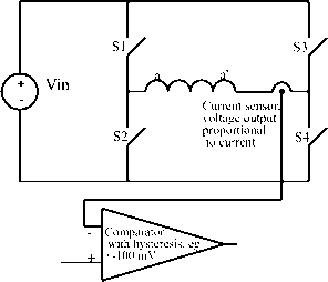

PWM logic signal output.

Turns on SI and S4 if high (current below reference), or S2 and S3 if low (current above reference)

Current

PWM Logic output signal

/ Desired I e/ current

ActuW currdnt

FIGURE 27.64 Hysteresis-band current control and PWM waveforms.

The general process of controlhng by switching a voltage fully on or fully off at high speed is called pulse-width modulation (PWM), and the specific method of current control achieved here with PWM is called hysteresis band current control (HBCC). Of course, to keep this current ripple small, the switching may need to be very fast, but with modern semiconductor switches there is no great problem up to 100 kHz for small machines and typically above 15 kHz for acoustic noise reasons, for machines rated up to several hundred kilowatts.

A perceived drawback of HBCC is that the switching frequency is determined by circuit inductance, the width of hysteresis band, the back emf, and the apphed voltage, ranging very widely in normal operation. It is not difficult, but it is a little more complicated, to use a fixed frequency and a hnear analog of the current error to modify the pulse width of the PWM signal.

27.6.3.1 Switching Losses

There is a practical limit to how often semiconductor switches can be operated. At every change of state, if the switch is carrying current as it is opened, then as the voltage rises across the switch and the current through it falls, there is a short pulse of power dissipated in the switch. Similarly, as the switch is closed, the voltage will take some time to fall and the current will take some time to rise, again producing a pulse of power dissipation. This loss is called switching loss. Fairly obviously, it will represent a power loss proportional to the switching frequency, and so the switching frequency is generally set as low as it can be without impinging on the effective operation of the circuit. Effective operation might well include criteria for acoustic noise and levels of vibration.

27.6.3.2 High-Efficiency Method of Managing Switching in the H Bridge

A very common way to control the current with the smallest number of switching transitions is to combine HBCC with, for example, alternating only SI and S2 in Fig. 27.65, leaving S4 on all the time, on the understanding that there will be a back emf in the winding and the current can still be increased or decreased as desired.

Thus, when the motor is rotating and the back emf is somewhere between zero and the rail voltage, alternating two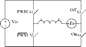

FIGURE 27.65

back emf.

H-bridge switching with one switch steadily on and a

switches rather than four will still allow current control in the coil, using for example HBCC, exactly as before.

This is a very common control scheme and will need some extra logic to reverse the direction of rotation of the motor, by either turning S4 off and S3 on continuously, or by swapping the control signals to the left and right legs. For full servo operation, normal H-bridge switching can be used and the logic is slightly different, but not significantly more comphcated. However, following the discussion above, the switching losses will be higher.

27.6.4 A Complete Controller

27.6.4.1 Combining Commutation and PWM Current Control

The real breakthrough is that one set of six switches can be used for both PWM and commutation. That is the clever part, and also the confusing part when one first tries to understand what is going on.

Thus, in a controller there are two control loops. The first is an inner current loop switching at, for example, 15 kHz to control carefully and exactly the current in two of the coils. Then at a much lower rate, for example at 50 times a second at 3000 rpm, the two coils doing the work are changed according to Table 27.2, controlled by an outer commutation loop, using information from the Hall-effect shaft-position sensors.

A complete controller is shown in block diagram form in Fig. 27.66. Various aspects of this block diagram will now be examined and explained in detail.

27.6.4.2 Hardware Details

27,6,4,2,1 Semiconductor Switches The three most likely semiconductor switches for a six-step controller are the bipolar junction transistor (BJT), the metal oxide silicon field-effect transistor (MOSFET), and the insulated-gate bipolar transistor (IGBT). Older controllers used BJTs; however, contemporary controllers tend to use MOSFETs for lower voltages and powers and IGBTs for higher voltages and powers. Both of these devices are controlled by a gate signal

Desired current (torque) command

fYate drives Gl to G6 -

Analog and Digital Signal Processing

Current sensors

Hall Effect Shaft Position Sensors

FIGURE 27.66 A complete controller showing the two feedback paths, one for the position sensors and one for the current sensors.

and will turn on when the voltage of the gate above the source or emitter is greater than about 5 V (about 10 V is common) and off when the gate voltage faUs below the threshold. Systems typically use zero volts for the off state. The controller of Fig. 27.66 shows MOSFETs used for the six switches.

The trick is that the voltage at terminal a, also Sis source, is either ground or the positive potential of the battery, depending on which switches are on. Driving S2, S4, and S6 is easy since the MOSFET sources are aU at the potential of the negative rail and the lower gate drive signals are referred to this rail.

There is a range of dedicated integrated circuits that can drive the switches SI, S3, and S5 and that use a charge pump principle to generate the drive signal and the drive power internally, all related to the MOSFET source potential. Various approaches to this technical challenge of providing a floating gate drive are commonly discussed under the generic heading of high-side drives.

For the most sophisticated drives, a transformer coupling is used to provide a tiny power supply especially for the isolated gate drive and to send the control signals through either an opto coupler or a separate transformer coupling. The high-side drive problems here are exactly the same as those encountered in the traditional buck converter, or in drives for induction motors and PMSMs.

27,6,4,2,2 Dead Time and Flyback Diodes Two issues have been mentioned that must be addressed when using highspeed electronic switches in inductive circuits.

The first, in Section 27.6.2, Electronic Commutation, was that care should be taken to ensure that the upper and lower switches in the same leg, (e.g., SI and S2) are never turned on at the same time. If the controUer attempts to turn one off

and the other on at the same instant and switch turn-off is slower than turn-on (as it is with BJTs and IGBTs), then a short circuit wiU result for a brief time. The bus capacitor is usually very large to provide ripple current (see later) and usually of very high quality, being fabricated especially for power electronic applications, and can easily provide thousands of amperes for a few microseconds, which is enough to destroy the semiconductor switches.

The second issue, discussed in Section 27.6.3, Current/ Torque Control, is that one cannot turn off both switches in a leg at the same time, even for a few nanoseconds, since the voltages resulting from attempting to interrupt current in an inductor wiU cause avalanche breakdown and failure of the semiconductors. This sounds like quite a dUemma.

There is actually a very simple and effective solution. At any transition the control circuitry ensures that the active switches are aU turned off before any switch is turned on, usually for a few microseconds. This is known as dead time, and its provision is an essential part of most of the dedicated integrated circuits in use. Then a flyback / freewheel diode is put in antiparaUel with each semiconductor switch, and this provides the current path during dead time. These diodes are shown in Fig. 27.66.

The diode has a little more loss than the switch, since the diode forward drop is more than the switch drop. This is significant in a low-voltage controUer. Fiowever, as stated earlier, for a low-voltage controUer MOSFETs are the device of choice. They have a lesser-known property: When gated on, they can carry current in both directions. Intriguingly, the on -state resistance is lower in reverse than in the forward direction! Thus, for low-voltage controllers, when the switch forward drop represents a significant contribution to losses, the MOSFET is turned on after dead time for both current

PWM Logic оифи! signal

I up

Logic

signal

I down

Logic

signaj

lime

i- 1

FIGURE 27.67 Dead time introduced into the PWM logic signal, for switch drive.

directions. Thus, the higher loss in the diode is only for a few microseconds.

It is not difficult to produce from the PWM signal an / up logic signal that is used to cause the current to increase and an / down logic signal used to decrease it, with the timing as shown in Fig. 27.67. The function can be executed in sequential logic, or with simple analog timing circuits.

27.6.4.2,4 The Smoothing Capacitor on the Input to the Controller This is a substantial capacitor, often very expensive (it is shown in Fig. 27.66 as С in), and its design is quite challenging. The issue of smoothing is quite serious. If there are high-frequency or sudden current changes in the leads from the dc supply to the controller, they will radiate electromagnetic energy. Good design will limit the length of conductors in which current is changing rapidly. Thus, a very large capacitor is placed physically as close to the positive bus of the switches as possible, aiming to have steady current in the longer conductors from the dc supply up to the capacitor. When the motor is running at, say, half speed and providing large torques, a very high level of ripple current is carried by this capacitor. Kirchhoffs current law (KCL) must be apphed at node A, as shown in Fig. 27.68. Good capacitors have a maximum ripple-current rating buried in their specification sheets. It turns out that in general, the size of the capacitor in a given design has very little to do with how much voltage ripple one can tolerate at the bus but rather is determined by the ability to carry the ripple current without the capacitor heating up and failing. It has been known that small electro-lytics in prototype controllers mysteriously explode. On searching it is found that they are in parallel with the main capacitor and quite close to it, so they carry a lot of ripple current, then heat up and explode!

27.6.4.2.3 Semiconductor Detail In MOSFETs and most IGBTs, there is a diode already within the device; it is unavoidable and results from the fabrication processes. In modern power semiconductors, this intrinsic diode is optimized to be a good switching diode. The serious designer, however, will check the specifications for reverse recovery of this diode, since in highly optimized controller designs, reverse recovery losses in the intrinsic diode can be significant and are very difficult to control. In low-voltage controllers one can put a Schottky diode in parallel with the intrinsic body diode. The Schottky diode, with its lower forward voltage drop will tend to take the current and has no reverse recovery problems, but the current must commutate to it from the semiconductor die, and the inductance of the connections is critical.

27.6.4.3 The Signal-Processing Block for Producing Switch-Drive Signals from Hall-Effect Sensors and Current Sensors

27.6.4.3.1 Operation of the Hall Sensors The flux density directly under a magnet pole can be any where from 500 to 800 mT with NdFeB magnets. Hall effect (HE) sensors with a digital output, called Hall-effect switches, change state at very close to zero flux density. Thus, they will change state when the north and south pole are equidistant from them, so that for example, in Fig. 27.69, the switch HEl is just changing state with the rotor as shown.

In practice a motor designer needs to consider what magnetomotive force comes from the current in the windings

I supply

I controller

I capacitor

To controller switches

-1>