current and flux-producing stator current) can be achieved as shown in Fig. 28.4(a).

In Fig. 28.4 the gating signals of the six inverter switching devices are obtained on the output of hysteresis current controllers. On the inputs of these the difference between the actual (measured) and reference stator line currents are present. The three-phase stator current references are obtained from their two-axis components (4d5 4q) the application of the two-phase-to-three-phase (2 3) transformation, and these are obtained from the reference values of 4d5 4q y the apphcation of the exp(j0j.) transformation. These reference values are obtained in the appropriate estimation block from the reference value of the torque (tgj.gf) and the monitored rotor speed (coj. This estimation block can be implemented in various ways, according to the required control strategy. In general there are three different constant angle control strategies: fastest torque control, maximum torque/ampere control and maximum power factor control. It can be shown [35] that, for example, the fastest torque response can be obtained by a controller, where у = 1ап~ {LJL where у is the angle of the stator current space vector with respect to the real-axis of the rotor reference frame {d axis), as shown in Fig. 28.4(b). The rotor-oriented control scheme of the synchronous reluctance machine shown in Fig. 28.4(a) is very similar to the rotor-oriented control scheme of the permanent magnet synchronous machine shown in Fig. 28.3(a).

It should be noted that in a recent book [35] more than 20 types of sensorless vector drives have been discussed in detail.

28.2.2 Fundamentals of

Direct-Torque-Controlled Drives

In addition to vector control systems, instantaneous torque control yielding very fast torque response can be obtained by employing direct torque control. Drives with direct torque control (DTC) are finding great interest, since ABB recently introduced the first industrial direct-torque-controUed induction motor drive, which according to ABB can work even at zero speed. This is a very significant industrial contribution, and it has been stated by ABB that direct torque control (DTC) is the latest ac motor control method developed by ABB [31, 35].

ABB has recently introduced a DTC based medium voltage drive called the ACS 1000 equipped with Sinus Filter, thus feeding pure sinusoidal voltages and currents to the motor. This is ideal for pumps and fans, particularly for retrofits.

ABB has also recently introduced a DTC based current excited synchronous machine drive caUed the ACS6000 SD. This is particularly suitable for medium voltage metal roUing miU applications.

In a DTC drive, flux linkage and electromagnetic torque are controlled directly and independently by the selection of optimum inverter switching modes. The selection is made to restrict the flux linkage and electromagnetic torque errors

within the respective flux and torque hysteresis bands, to obtain fast torque response, low inverter switching frequency and low harmonic losses. The required optimal switching voltage vectors can be selected by using a so-caUed optimum switching voltage vector look-up table. This can be obtained by simple physical considerations involving the position of the stator flux linkage space vector, the avaUable switching vectors and the required torque and flux hnkage.

Figure 28.5 shows the schematic of one simple form of a DTC induction motor drive, which uses the stator flux linkages. Thus it wiU be referred to as a stator-flux-based DTC induction motor drive, but other forms of DTC drives are also possible, which are based on the rotor flux linkages or magnetizing flux linkages.

In Fig. 28.5 the induction motor is supplied by a VSI inverter and the stator flux linkage and electromagnetic torque errors are restricted within their respective hysteresis bands. For this purpose a two-level flux hysteresis comparator and a three-level torque hysteresis comparator are used respectively. The outputs of the flux and torque comparators {d\i/, dt) are used in the inverter optimal switching table, which also uses information on the position (p) of the stator flux hnkage space vector. It should be noted that it is not the actual flux linkage vector position which has to be determined, but only the sector where the flux linkage vector is located. It can be seen that the DTC drive scheme requires stator flux linkage and electromagnetic torque estimators. In principle, the stator flux linkages can be estimated by integrating the terminal voltage reduced by the ohmic losses. Fiowever, at low frequencies large errors can occur due to the variation of the stator resistance, integrator drift and noise. Therefore, instead of using open-loop flux linkage estimators, other techniques should be used (e.g. flux observer). Observers have reduced sensitivity to parameter variations, but the accuracy of a stator flux linkage observer can be increased by also using onhne parameter estimators (e.g. for the estimation of the stator resistance), or a thermal model of the machine whose outputs can be used for accurate stator resistance estimation. Fiowever, it is also possible to use a joint state and parameter observer which estimates the stator flux linkages, the stator resistance or temperature (required to estimate the hot value of the stator resistance), and also the rotor speed (in a sensorless drive).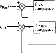

Electromagnetic torque

flux linkage estimator

FIGURE 28.5 Schematic of stator-flux-based DTC induction motor drive.

For stator flux linkage estimation it is not necessary to monitor the stator voltages since they can be reconstructed by using the inverter switching functions and the monitored dc link voltage (see also Section 28.2.3.2).

The main features of the DTC can be summarized as: direct control of stator flux and electromagnetic torque; indirect control of stator currents and voltages; approximately sinusoidal stator stator fluxes and stator currents; reduced torque oscillations; excellent torque dynamics; inverter switching frequency depends on flux and torque hysteresis bands. The main advantages of a conventional DTC are: absence of coordinate transformations (which are required in most of the vector-controlled drive implementations); absence of separate voltage modulation block (required in vector drives); absence of voltage decoupling circuits (required in voltage-source inverter-fed vector drives), reduced number of controllers (e.g. only a speed controller is required if the drive contains a speed loop), the actual flux hnkage vector position does not have to be determined, but only the sector where the flux linkage is located, etc. However, in general, the main disadvantages of a conventional DTC can be: large torque and flux ripples and variable switching frequency. Measurements on ABB ACS600 DTC drives prove that in ABBs DTC implementation these problems are solved. In general, these problems can be overcome by using suitable techniques: DTCs exist with torque and flux ripple minimization schemes [35, 41], and although the variable switching frequency is caused by the hysteresis control of the electromagnetic torque and stator flux linkage, smaller torque and flux hysteresis widths result in a smoother harmonic spectra.

In the ABB DTC induction motor drive, torque response times typically better than 2 ms are obtained together with high torque control linearity even down to low frequencies including zero speed. According to ABB, the new ac drive technology rests chiefly on a new motor model which enables the computation of motor states without using a speed or position sensor. There is only hmited information on the ABB ACS600 motor model. The ABB DTC induction motor drive contains the ACS 600 frequency converter (inverter), shown in Fig. 28.6. The inverter switchings directly control the motor flux linkages and electromagnetic torque.

The ACS 600 product family suits many applications and operating environments, with a large selection of ac voltage, power and enclosure ratings, combined with highly flexible communication capabilities. For illustration purposes Fig. 28.7 shows some measured responses obtained in the ABB sensorless DTC induction motor drive (see also Section 28.2.3, which discusses various speed-sensorless implementation techniques, including the sensorless technique used by ABB).

ABB has also developed a DTC induction motor drive, which combines accurate speed control and direct torque control with line braking for regenerative applications, such as cranes, centrifuges and winding machines in the range ll-50kW. The ACS 611 incorporates two inverters in one

FIGURE 28.6 ACS 600 frequency converter (Courtesy of ABB Industry, Oy, Helsinki).

frame. An active inverter replaces the usual diode rectifier (at the input side), thus reducing time harmonics and ensuring an almost perfectly sinusoidal supply. The extra inverter also enables full four-quadrant operation and two-way energy flow, which means that the drive can divert excess energy from a braking motor back into the electrical system, when it is not required by the motor. The DTC technology allows the drive to switch between maximum motoring and maximum generating power in less than five milliseconds, allowing the drive to adapt to highly dynamic changes of the motor load.

Regenerative DTC based ACS600 Multidrive is also available from 200 kVA to 4000 kVA.

It should be noted that basically there are two types of DTC drives: conventional DTC drives, where the switching frequency is changing, and DTC drives, with constant switching frequency [35]. It can be shown [40, 41] that in this second type of DTC drive it is relatively easy to ensure reduced torque ripples. For the ACS600 the average switching frequency is controlled.

Other types of DTC drives utilize similar principles to those discussed above, i.e. direct-torque-controlled permanent magnet synchronous machine drives, direct-torque-controlled synchronous reluctance motor drives and direct-torque-controlled electrically excited synchronous motor drives. A recent book [35] discusses 10 types of induction motor and synchronous motor DTC drives, and for this purpose both the voltage-source and current-source inverter-fed drives (VSI, CSI) are considered.

It is important to emphasize some differences between the direct torque control of an induction motor and that of a permanent magnet synchronous motor. For permanent magnet synchronous motors the initial values of the stator flux hnkages (in the stationary reference frame) are not zero.

Estimated air-gap torque 11r-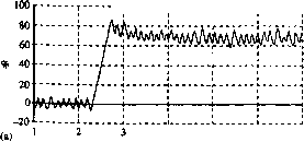

Phase current

80 rijlltf

60 40 20 0 -20 -40 -60

Time (ms) - Shaft torque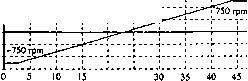

20 25 Time (s)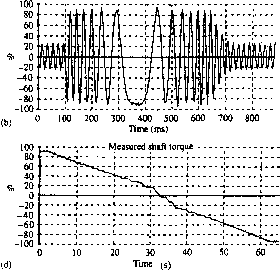

2 1.5 1

0 -0.5 -1 -1.5 -2

г - Estimated mechanical speed - л

40 60

Time (ms)

FIGURE 28.7 ABB sensorless DTC drive responses.

Furthermore, in a permanent magnet synchronous motor, the stator flux hnkage space vector wiU change even when zero vohage vectors are apphed, since the magnets rotate with the rotor. In addition, it foUows from Eqn. (28.5) that, e.g., for the permanent magnet synchronous motor with surface-mounted magnets the electromagnetic torque is proportional to the load angle and not to the slip frequency as in induction motors (the load angle is defined as the angle between the stator and rotor flux linkage space vectors, when the stator resistance is neglected). This is why for controUing the amplitude of the stator flux linkage space vector and for changing the electromagnetic torque (or torque angle) quickly, zero voltage vectors are not used in the direct-torque-controUed permanent magnet synchronous motor drive. The fastest torque response in the permanent magnet synchronous motor drive employing DTC can be obtained by increasing the rotating speed of the stator flux linkage space vector.

28.2.3 Speed and Position Sensorless ac Drive Implementations

In the present subsection, the general aspects of sensorless drives are first discussed. This is followed by discussing the main types of sensorless high-performance ac drive schemes.

28.2.3.1 General, Objectives, Main Types of Sensorless Schemes

In the past few years great efforts have been made to introduce speed and/or shaft position sensorless torque-controlled (vector- and direct-torque-controUed) ac drives. These high-performance drives are usually referred to as sensorless drives, although the terminology sensorless refers only to the speed and shaft sensors, and there are stiU other sensors in the drive system (e.g. current sensors), since closed-loop operation cannot be performed without them.

Sensorless vector drives have become the norm for industry and almost every large manufacturer. Fiowever, it is a main feature of almost aU of these industrial drives that they cannot operate at very low frequencies without speed or position sensors. In general, to solve the problems at low frequencies, a number of special techniques can be used, e.g. which deliberately introduce asymmetries in the machine, or where extra signals are injected into the stator in order to detect various types of anisotropics (due to slots, saturation, etc.). Fiowever, so far these techniques have not been accepted by industry, due to the undesirable side effects and other problems [43].

To reduce total hardware complexity and costs, to increase the mechanical robustness and rehability of the drive, to have increased noise immunity, to eliminate cables connecting the

mechanical sensors to other parts of the drive, to reduce the overall size, etc., it is desirable to ehminate the conventionally used mechanical (speed, position) sensors in high-performance drives. Furthermore, an electromechanical sensor increases system inertia, which is undesirable in high-performance drives. It also increases the maintenance requirements. In very small motors it is impossible to use electromechanical sensors. In a low-power torque-controlled drive the cost of such a sensor can be almost equal to all the other costs. In drives operating in hostile environments, or in high-speed drives, speed sensors cannot be mounted. As realtime computation (DSP) costs are continuously and radically decreasing (see also Section 28.3 on low-cost Texas Instruments motion control DSPs), speed and position estimation can be performed by using software-based state-estimation techniques where stator vohage and/or current measurements are performed.

The main techniques of sensorless control for induction motor drives [35, 43], which can be used for both vector-controlled and direct-torque-controlled drives are:

1. open-loop estimators using monitored stator voltages/ currents

2. estimators using spatial saturation stator phase third harmonic voltage

3. estimators using saliency (geometrical, saturation, etc.) effects

4. model reference adaptive systems (MRAS)

5. observers (Kalman, Luenberger)

6. estimators using artificial intelligence (artificial neural network and fuzzy-logic-based estimators, fuzzy-neural estimators, genetic-algorithm-assisted neural networks, etc.).

The main techniques of sensorless control of vector-controlled and direct-torque-controlled permanent magnet synchronous motor drives are [35, 43]:

1. open-loop estimators using monitored stator voltages/ currents

2. stator phase third harmonic voltage-based position estimator

3. back emf-based position estimators

4. observer-based (Kalman, Luenberger) position estimators

5. estimators based on inductance variation due to geometrical and saturation effects

6. estimators using artificial intelligence (artificial neural networks, fuzzy-logic-based systems, fuzzy-neural networks, etc.).

The main techniques for sensorless control of synchronous reluctance motors are [35]:

1. estimators using stator voltages and currents, utilizing speed of stator flux linkage space vector

2. estimators using spatial saturation third harmonic voltage component

3. estimators based on inductance variation due to geometrical effects:

indirect position estimation using the measured rate of change of the stator current (no test voltage vector used)

indirect flux detection by using measured rate of change of the stator current and applying test voltage vectors/on-line reactance measurement (INFORM) method/low-speed apphcation

indirect position estimation using the rate of change of the measured stator current vector by using zero test voltage vector (stator is short-circuited) high speed application

4. estimators using observers (e.g. extended Kalman filter)

5. estimators using artificial intelligence (neural networks, fuzzy-logic-based systems, fuzzy-neural networks, etc.).

In addition to the sensorless techniques shown above, it is also possible to implement quasi-sensorless (encoderless) drives, which do not contain conventional speed or position sensors, but where the speed and position information is obtained by using a sensor bearing. For this purpose SKF has developed a family of sensor bearings, and it has been shown [39, 40] that these can also be used in high-performance drives.

The latest field of research in sensorless drives is related to the sensorless position control of induction motors at very low and zero speed. This involves zero speed operation at a predetermined rotor position. In this case the control algorithm must rely on some anisotropic effects (e.g. rotor slotting).

28.2.3.2 Sensorless Drive Schemes

In the present section, various sensorless ac drive schemes are discussed together with encoderless (quasi-sensorless) drive schemes.

28,2,3,2,1 Mathematical-Model-Based Schemes Due to page restrictions only some of the main principles will be discussed briefly.

Open-Loop Flux Estimators Using Monitored Stator Voltages/ Currents, Voltage Reconstruction, Drift Compensation Many types of open-loop and closed-loop flux hnkage, position and speed estimators have been discussed in detail in a recent book [35]. The position-sensorless estimators discussed first are open-loop estimators. If the open-loop estimator is a stator flux linkage estimator, then it will also yield the angle of the stator flux linkage space vector with respect to the real axis of the stator reference frame (p), together with the modulus of the flux space vector. In general, for a synchronous machine.

in the steady state, the first time derivative of this angle gives exactly the rotor speed, ш^. = dpjdt, so accurate estimation of the stator flux vector also yields the rotor speed, and this concept can be used in speed-sensorless synchronous motor drives. However, in the transient state, in a drive where there is a change in the reference electromagnetic torque, the stator flux linkage space vector moves relative to the rotor (to produce a new torque level), and this influences the rotor speed. This effect can be neglected if the rate of change of the electromagnetic torque is hmited.

Open-loop flux estimators can use either a voltage model or a current model: these two cases are now discussed. If a voltage model is used, in general, the stator flux linkage space vector can be obtained by the integration of the terminal voltage minus the stator ohmic drop:

(щ - RX)dt.

(28.12)

The voltage space vector {щ) and the current space vector (4) are obtained from measurements of the stator voltages and stator currents. Thus the direct- and quadrature-axis stator flux linkage components in the stator reference frame are obtained as

(4d - s4d) (4q - s4q)

(28.13) (28.14)

where the stator voltages and currents can be obtained from the measured hne voltages and currents as foUows:

4d - 3 (ba ~ %c)

4q = (-1/V3)(wac - %a)

4d = 4a

4Q = (l/V3)(4A + 2isB)

(28.15) (28.16) (28.17) (28.18)

If the stator flux linkage components are known, e.g. they have been obtained by using Eqns. (28.13), and (28.14), then it is also possible to estimate the components of the rotor flux linkage space vector by considering \}/[ = (Ц/Ь^Хф - VJ), where ф[ is the space vector of the rotor flux linkages expressed in the stationary reference frame, ф[ = ф^ -h ]фщу and Lj. are the magnetizing inductance and rotor self-inductance respectively, and is the stator transient inductance, Lg = crLg, where the leakage factor is cr = [1 - 1/(44)], where 4 is the stator self-inductance. Thus in component form, ф^ = (Ц/Ь^ф^ - L;4d) and ф^ = (Ц/L)(ф^Q - Ts4q)- It can be seen that the estimation of the stator flux linkage space vector requires integration, and also the stator resistance. The presence of the integrator and the temperature dependency of the stator resistance makes this

open-loop estimator impractical at very low stator frequencies (see also below), if some modifications are not made to the estimator.

If the so-caUed current model is used for the estimation of the various flux linkages, then, e.g., for an induction motor the rotor voltage equation is utUized for the estimation of the rotor flux linkage space vector. It then foUows from the rotor voltage space vector equation of the induction motor and also by using the defining equations for the stator and rotor flux linkage space vectors that

dф[/dt = -(l/nWr + (LJT,)l +]со,ф[ (28.19)

where Т/ is the rotor transient time constant (Т/ = сгТ^., where Tj. = LJRj. is the rotor time constant). However, it can be seen that this estimator also requires the speed signal (or a position signal), so this is not a sensorless solution. On the other hand, it also foUows that this estimator even works at zero frequency, but is sensitive to the detuning of the machine parameters and Tj., which can change due to main flux saturation and temperature effects. To get higher accuracy, parameter adaptation must be used (where the parameters are adapted in realtime).

In comparison, the voltage-model-based flux estimator performs better at higher speeds, since in this case the stator resistance has reduced effects (since the ohmic voltage drop is smaU). However, at lower speeds, the current-model-based flux estimator performs better, since it can work even at zero frequency, but as mentioned above, it requires a speed or position estimator and is also sensitive to various machine parameters. It foUows that a hybrid observer (hybrid model), which uses both the voltage-model-based and current-model-based estimators could be used for flux estimation in the entire speed range, but this is not a sensorless solution.

The angle of the stator flux hnkage space vector can be obtained from the stator flux hnkage components as

Ps = tan HAsq/Asd)-

(28.20)

It is important to note that, e.g., in a vector-controUed induction motor drive using stator flux-oriented control, or in a direct-torque-controUed induction motor drive, and also in a vector-controUed PMSM drive with surface magnets, or in a direct-torque controlled PMSM drive using Eqn. (28.30), depends greatly on the accuracy of the estimated stator flux linkage components and these depend on the accuracy of the monitored voltages and currents, and also on an accurate integration technique. Errors may occur in the monitored voltages and currents due to the foUowing factors: phase shift in the measured values (because of the sensors used), magnitude errors because of conversion factors and gain, offset in the measurement system, quantization errors in the digital system, etc. Furthermore, an accurate value has to be used for

the stator resistance, especially if the drive operates at low stator frequency. In general, for accurate flux linkage estimation, the stator resistance must be adapted to temperature changes [43]. The integration can become problematic at low frequencies, where the stator voltages become very small and are dominated by the ohmic voltage drops. At low frequencies the voltage drop of the inverter must also be considered [43]. This is a typical problem associated with voltage-model-based open-loop flux estimators used in all ac drives, which utilize monitored terminal voltages and currents.

Drift compensation is also an important factor in a practical implementation of the integration, since drift can cause large errors of the position of the stator flux linkage space vector. In an analog implementation the source of drift is the thermal drift of analog integrators. However, a transient offset also arises from the dc components which result after a transient change. An incorrect flux angle will cause phase modulation in the control of the currents at fundamental frequency, which, however, will produce an unwanted fundamental frequency oscillation in the electromagnetic torque of the machine. Furthermore, since in the open-loop speed estimator which utilizes the stator flux linkage components, the rotor speed is determined from the position of the stator flux linkage space vector, thus a drift in the stator flux linkage vector will cause incorrect and oscillatory speed values. In a speed control loop, this drift error, will cause an undesirable fundamental frequency modulation of the modulus of the reference stator current space vector (I4ref !) The open-loop stator flux linkage estimator can work well down to 1-2 Hz, but not below this, unless special techniques are used. In addition to the stator flux estimation based on Eqns. (28.13) and (28.14), and which is shown in Fig. 28.8(a), it is also possible to construct other stator flux linkage estimators, where the integration drifts are reduced at low frequency. For this purpose, instead of open-loop integrators, closed-loop integrators can be used [35].

1 + /?T

R-*P

<! (b)

FIGURE 28.8 Stator flux linkage estimators, (a) Estimation in the stationary reference frame, (b) estimation in the stationary reference frame using quasi-integrators.

It is also possible to estimate the stator flux linkage components by using low-pass filters instead of pure integrators. In this case l/p is replaced by T/(l +pT) where T is a suitable time constant. Such a flux hnkage estimation scheme is shown in Fig. 28.8(b). To obtain accurate flux estimates at low stator frequency, the time constant T has to be large and the variation of the stator resistance with temperature also has to be considered. It is an advantage of using the flux linkage estimation scheme shown in Fig. 28.8(b) that the effects of initial conditions are damped by the time constant T. Obviously there will be a phase shift between the actual and estimated flux linkages, but increased T decreases the phase shift. However, an increased T decreases the damping.

In vector-controlled and DTC drives it is also possible to use such improved low-pass-filter-based flux estimators, where the magnitude and phase errors introduced by the low-pass-filter are reduced. For example, in a DTC voltage-source inverter-fed induction motor drive the inaccurate flux estimation can lead to incorrect voltage switching vector selection, but the application of an improved low-pass-filter-based flux estimator can lead to reduced current harmonics, reduced torque ripples in the steady state and also to an improved stator flux locus. For this purpose, in the improved flux estimator, in addition to the low-pass filter (which acts on the stator voltage minus ohmic drops), there is an extra compensator circuit, which is connected to the output of the low-pass filter. This compensator adds to the direct-axis stator flux the extra value (co/cOg) times the quadrature-axis stator flux (which is the first output of the low-pass filter), and it adds to the quadrature-axis stator flux the value {(d/cd) times the direct-axis stator flux (which is on the second output of the low-pass filter), where (co/cOg) is the ratio of the cutoff frequency of the low-pass filter and the synchronous frequency. The synchronous frequency can be obtained by using the monitored (or reconstructed) stator voltage, stator current and by also knowing the stator resistance.

The estimation of the stator flux linkage components described above requires the stator terminal voltages. However, it is possible to have a scheme, where these voltages are not monitored, but they are reconstructed from the dc link voltage (Uj) and the switching states (5д, Sg, Sq) of the six switching devices of a six-step voltage-source inverter [35, 36]. Figure 28.9 shows the schematic of the six switches of the voltage-source inverter and the values of the switching func-

r r r-

tions are also shown together with the appropriate switch positions.

The stator voltage space vector (expressed in the stationary reference frame) can be obtained by using the switching states and the dc link voltage Uj as

4=fd(5A + 5B + a2Sc). (28.21)

Thus

= Re(a23)=il/d(-SA + 2SB-Sc)

(28.22) (28.23)

= Ке(а-щ) = i Ui-Sj, - Sb + 2Sc) (28.24)

Hence by the substitution of Eqn. (28.21) into (28.12), the stator flux linkage space vector can be obtained as foUows for a digital implementation. The kth sampled value of the estimated stator flux linkage space vector (in the stationary reference frame) can be obtained as

ФД) = ФД - 1) + f U,T[S(k - 1) + aS(k - 1)

+ aSc(k-l)]-Rjl(k-l)

(28.25)

where T is the samphng time (flux control period), 4 is the stator current space vector. Resolution of Eqn. (28.25) into its real and imaginary axis components gives ij/j) and xJ/q. However, it is important to note [43] that Eqn. (28.25) is sensitive to:

voltage errors caused by dead time effects (e.g. at low speeds, the pulsewidths become very smaU and the deadtime of the inverter switches must be considered)

the voltage drop in the power electronic devices

the fluctuation of the dc link voltage

the variation of the stator resistance (but this resistance variation sensitivity is also a feature of the method using monitored stator voltages).

of the inverter is not equal to the desired (reference) voltage space vector, but it is equal to the sum of the desired voltage space vector and an error voltage space vector (Ащ). The error voltage space vector can be estimated by utUizing information avaUable on the switching times of the power transistors. Various dead-time compensation schemes have been discussed in [35] and, for example, it is possible to implement such dead-time compensation schemes where the existing space vector PWM strategy is not changed but only the reference stator voltage space vector (Щге{) is modified by adding the error stator voltage space vector.

Recent trends are such, that in position-sensorless drives, the stator voltage sensors are also eliminated and only current sensors are used, but the dc hnk voltage is also monitored. It is possible to have a position-sensorless drive implementation based on Eqn. (28.25) where the dead-time effects are also considered and the thermal variation of the stator resistance is also incorporated into the control scheme, which wiU even work at very low speeds. Obviously there are other possibUities as weU to solve the problem of integration at low frequencies, e.g. cascaded low-pass filters can be used with programmable time constants, etc. Sometimes it is also possible to use appropriate voltage references instead of actual voltages if the switching frequency of the inverter is high compared to the electrical time constant of the motor. In this case the appropriate reference voltages force the actual currents to foUow their references. Such a solution has the additional advantage of further reducing the required number of sensors, and since no filtering of the voltages is required, no delay is introduced due to filtering. In general, a delay introduced by a low-pass filter (acting on the voltages) is a function of the motor speed (since the modulus of the voltage is a direct function of the speed, e.g. at low speeds it is smaU), thus in a vector-controUed drive it is not possible to keep the stator current in the desired position, as speed changes. This adversely affects the torque/ampere capability and motor efficiency, unless filter-delay compensation is introduced (e.g. by using a lead-lag network).

Due to the finite turnoff times of the switching devices (power transistors) used in a three-phase PWM VSI, there is a need to insert a time delay (dead time, tjj) after switching a switching device off and the other device on in one inverter leg. This prevents the short-circuit across both switches in the inverter leg and the dc link. Due to the presence of the dead-time, in a voltage controUed drive system, the amplitude of the output voltages of the inverter (stator voltages of the machine) wiU be reduced and wiU be distorted. This effect is very significant at low speeds. In space vector terms this means that at very low speeds, the stator voltage space vector locus produced by the inverter, without using any dead-time effect compensation scheme, becomes distorted and the amplitude of the stator voltage space vector is unacceptably smaU. Due to the presence of the dead time, the output voltage space vector

Open-Loop Speed Estimators In the previous subsection, open-loop flux estimators have been discussed for both induction motors and synchronous motors. In the present subsection it is shown that, if the stator flux linkages are known, then the rotor speed of the induction or synchronous motor can be simply obtained by utUizing the information on the speed of the stator flux linkage space vector.

For the synchronous machine (e.g. permanent magnet synchronous machine), the rate of change of the stator flux position angle, i.e. the first derivative of the angle p, is equal to the rotor speed (rotor speed is equal to stator flux vector speed), see also Eqn. (28.16):

cOj. = dpjdt.

(28.26)

Thus, for example, in the speed control loop of a permanent magnet synchronous motor drive, this relationship can be directly utilized. The estimation of the rotor speed based on the derivative of the position of the stator flux linkage space vector can be slightly modified by considering that the analytical differentiation, dpjdt, where = tan~(\l/Q/pj)% gives

cd, = (dJdt - iA3Q#3Q/t)/(iAd + iAq). (28.27)

In Eqn. (28.27) the derivatives of the flux linkage components can be ehminated, since they are equal to the respective terminal voltage minus the corresponding ohmic drop; thus:

(28.28)

is obtained. In Eqn. (28.28) the stator flux hnkage components can be obtained by using Eqns. (28.13) and (28.14). For digital implementation, Eqn. (28.28) can be transformed into

соД) = [ф,(к - 1)ф,(к) - ф,(к - 1Ж^,(к)]/[Т,(ф,(к) + AsqC))] (28.29)

where cdk) is the value of the speed at the kth samphng time, and Tg is the sampling time.

The rotor speed estimation based on the position of the stator flux linkage space vector can also be conveniently used in other schemes, i.e. stator-flux-oriented control of the permanent magnet synchronous machine or in vector-controlled or direct-torque-controlled induction motor drives (e.g. in the case of the induction motor see below). However, in all of these applications, for operation at low speeds, the same hmitations hold as above. Furthermore, for the induction motor, dpjdt will not give the rotor speed, but will only give the speed of the stator mmfs, which is the synchronous speed (ш^), and the rotor speed is the difference between the synchronous speed and the slip speed (Шг = cd-cdJ.

In an induction motor drive, e.g. in the DTC induction motor drive, the speed signal can be required due to two reasons. One reason is that it can be used for stator flux linkage estimation, if the stator flux linkage estimator requires the rotor speed signal (e.g. when a hybrid stator flux linkage estimator is used, which uses both the stator voltage equation, and also the rotor voltage equation, and the rotor voltage equation contains the rotor speed). The other reason is that a rotor speed signal is required if the drive contains a speed control loop (in this case the speed controller outputs the torque reference, and the input to the speed controller is the difference between the reference speed and the estimated speed). In many variable-speed drive apphcations torque control is required, but speed control is not necessary. An

example of an application where the electromagnetic torque is controlled, without precise speed control, is traction drives. In traction applications (diesel-electric locomotives, electrical cars, etc.) the electromagnetic torque is directly controlled, i.e. the electromagnetic torque is the commanded signal, and it is not the result of a speed error signal.

The key to the success of simple open-loop speed estimation schemes is the accurate estimation of the stator (or rotor) flux linkage components. If the flux linkages are accurately known, then it is possible to estimate the rotor speed by simple means, which utilizes the speed of the estimated flux hnkage space vector. This technique is used in various commercially available induction motor drives; thus this is now briefly discussed. In these commercial implementations the stator voltages are not monitored but are reconstructed from the dc hnk voltage and switching states of the inverter (see above).

In an induction motor the rotor speed can be expressed as

(28.30)

where cd. is the angular speed of the rotor flux (relative to the stator), cOjj. = dpjdt, and cdi is the angular slip frequency. It follows from the induction motor equations [35] that

= [L/(Tr.A/)](-.Arq4D + Ard4Q)

or in terms of the electromagnetic torque

= (2tM/mk\)

(28.31)

(28.32)

where is the magnetizing inductance, T, is the rotor time constant, is the electromagnetic torque, is the rotor resistance, P is the number of pole pairs, and are the rotor flux hnkage components (in the stationary reference frame), \ф,\ is the modulus of the rotor flux hnkage space vector, \ф,\ = yjArd +Ащ) 4d and 4q are the stator direct and quadrature axis currents (in the stationary reference frame). Physically, cdi is the speed of the rotor flux hnkage space vector with respect to the rotor. It is possible to obtain an expression of cd. in terms of the rotor flux hnkage components by expanding the expression for the derivative dpjdt. Since the rotor flux linkage space vector expressed in the stationary reference frame is ф^, = ф, + ]ф, = \Фг\exp(iPr) thus = tan-iArq/Ard) it follows that

ш^г = dфJdt = d[tш-\ф,/ф,)]/dt

= {ф,dф,Jdt - ф,dфJdt)/{ф] + ф\). (28.33)

Substitution of Eqn. (28.33) into Eqn. (28.30) and by also considering Eqns. (28.31) or (28.32), gives

, = {ф,dф,Jdt - ф,dфJdt)/\ф^ -[LJт^ф^\фJ,-Ф,i,)

(28.34)

= (Ard#rq/ - dlijjdt) - (2tM/mh)

(28.35)

where the electromagnetic torque can be obtained from

te=P(ФsDhQ-ФsQhD) (28.36)

4 = f m/4)(Ard4Q - Arqd)-

(28.37)

When a rotor speed estimator is based on Eqn. (28.34) or (28.35), it uses the monitored stator currents and, e.g., the rotor flux components, which, however, can be obtained from the stator flux linkages by considering

ф, = (Ц/ЬЛф, - L;4d) (28.38)

.Arq = (4/IJ(AsQ-bs4Q) (28.39)

where Ц is the rotor self-inductance and Ц is the stator self-inductance. In Eqns. (28.36) and (28.37) the stator flux linkages can be obtained by using monitored stator currents and monitored or reconstructed stator voltages as discussed above, see Eqn. (28.25).

In summary it should be noted that the speed estimators discussed above depend heavily on the accuracy of the flux linkage components used. If the stator voltages and currents are used to obtain the flux estimates, then by considering the thermal variations of the stator resistance, (e.g. by using a thermal model), and also by using appropriate saturated inductances, the estimation accuracy can be greatly improved. However, a speed-sensorless high-performance direct-torque-controUed drive using this type of speed estimator wiU only work successfully at ultra low speeds (including zero speed), if the flux estimator is some type of a closed-loop observer.

Closed-Loop Observer-Based Flux and Speed Estimation in Vector and DTC Induction Motor Drives Full-Order Adaptive State Observers, Luenberger and Kalman Observers In general, an estimator is defined as a dynamic system whose state variables are estimates of some other system (e.g. electrical machine). There are basically two types of estimator: open loop and closed loop, the distinction between the two being whether or not a correction term, involving the estimation error, is used to adjust the response of the estimator. A closed-loop estimator is referred to as an observer. As discussed above, in open-loop estimators, especially at low speeds, parameter deviations have a significant influence on the performance of the drive both in the steady state and transient state. However, it is possible to improve the robustness against

parameter mismatch and also signal noise by using closed-loop observers.

An observer can be classified according to the type of representation used for the plant to be observed. If the plant is considered to be deterministic, then the observer is a deterministic observer, otherwise it is a stochastic observer. The most commonly used observers are Luenberger and Kalman types [35]. The Luenberger observer (LO) is of the deterministic type and the Kalman filter (KF) is of the stochastic type (of optimal oberserver). The basic Kalman filter is only applicable to hnear stochastic systems, and for non-linear systems the extended Kalman filter (EKE) can be used, which can provide estimates of the states of a system or both the states and parameters (joint state and parameter estimation). The EKE is a recursive filter (based on the knowledge of the statistics of both the state and noise created by measurement and system modeUing) which can be apphed to a non-hnear time-varying stochastic system. The basic Luenberger observer is apphcable to a hnear, time-invariant deterministic system. The extended Luenberger observer (ELO) is applicable to a non-linear time-varying deterministic system. The simple algorithm and the ease of tuning of the ELO may give some advantages over the conventional extended Kalman filter [35].

In high-performance induction machine drives it is possible to use various types of speed and flux observers. These include a fuU-order (fourth-order) adaptive state observer (Luenberger observer) which is constructed by using the equations of the induction machine in the stationary reference frame by adding an error compensator. This is a system which is also used in some commercial drives. Furthermore, the Extended Kalman Filter (EKE) and the Extended Luenberger Observer (ELO) could also be used [35], but at present, due to the large computational burden, these systems are not used in commercial drives. However, it should be noted that it is also possible to use reduced-order observers, where there is some reduction in computations. An EKF-based sensorless induction motor drive can also work at zero frequency [25].

In the fuU-order adaptive state observer the rotor speed is considered as a parameter, but in the EKE and ELO the rotor speed is considered as a state variable. Furthermore, as discussed above, whilst the ELO is a deterministic observer, the EKE is a stochastic observer which also uses the noise properties of measurement and system noise. When the appropriate observers are used in high-performance speed-sensorless torque-controlled induction motor drives (vector-controUed drives, direct-torque-controUed drives), stable operation can be obtained over a wide speed range. Various industrial ac drives already incorporate observers and it is expected that, in the future, observers wiU have an increased role in industrial high-performance vector and direct-torque-controUed drives.

Since at present, the adaptive state observer is the simplest observer used in high-performance drives, this is now described

briefly. However, for better understanding, first, a state estimator is described which can be used to estimate the rotor flux hnkages of an induction machine. This estimator is then modified so it can also yield the speed estimate, and thus an adaptive speed estimator is derived (to be precise, a speed adaptive flux observer is obtained). To obtain a stable system, the adaptation mechanism can be derived by using the state error dynamic equations together with Lyapunovs stability theorem [35]. In an inverter-fed drive system, the observer uses the monitored stator currents together with the monitored (or reconstructed) stator voltages, or reference stator voltages. However, when the reconstructed stator voltages or reference voltages are used, some error compensation schemes must also be used.

A state observer is a model-based state estimator, which can be used for the state (and/or parameter) estimation of a nonlinear dynamic system in realtime. In the calculations, the states are predicted by using a mathematical model (the estimated states are denoted by i), but the predicted states are continuously corrected by using a feedback correction scheme. This scheme makes use of actual measured states (x) by adding a correction term to the predicted states. This correction term contains the weighted difference of some of the measured and estimated output signals (the difference is multiplied by the observer feedback gain, G). Based on the deviation from the estimated value, the state observer provides an optimum estimated output value (x) at the next input instant. In an induction motor drive a state observer can also be used for the realtime estimation of the rotor speed and some of the machine parameters, e.g. stator resistance. This is possible since a mathematical dynamic model of the induction machine is sufficiently well known. For this purpose the stator voltages and currents are monitored on-hne and for example, the speed and stator resistance of the induction machine can be obtained by the observer quickly and precisely. The accuracy of the state observer also depends on the model parameters used. By using a DSP, it is possible to conveniently implement the adaptive state observer in real time. The state observer is simpler than the Kalman observer, since no attempt is made to minimize a stochastic cost criterion.

To obtain the full-order non-linear speed observer, first the model of the induction machine is considered in the stationary reference frame and then an error compensation term is added to this. The simplest derivation uses the stator and rotor space vector equations of the induction machine [35]. These yield the state variable equations in the stationary reference frame if the space vectors of the stator currents (4) and rotor flux linkages (i) are selected as state variables:

dx/dt = Ax-\-Bu

(28.40)

where the input matrix is В = [/2/5 2]- Furthermore, the output equation is defined as

In Eqn. (28.40) x = [4, ф[] is the state vector, which contains the stator current column vector, 4 = [4d 4q] and also the rotor flux linkage column vector, = [ф,, фщ]. Furthermore, и is the input column vector, which contains the direct and quadrature axis stator voltages u = щ = [щ^) Що The state matrix A is a 4 x 4 matrix and is dependent on the angular rotor speed (coj, I2 is a second-order identity matrix, /2 = diag(l, 1), and O2 is a two-by-two zero matrix. In Eqn. (28.41) С is the output matrix, С = [I2, Оз]. Equation (28.40) can be used to design the observer and for this purpose the correction term described above is added (this contains the difference of actual and estimated states). Thus a full-order state observer, which estimates the stator currents and rotor flux linkages can be described as

dx/dt = Ax-\-Bu-\- G(4 - 4)

--[1/t; + (1 - (7)/t;]/2 [ьль^ьж/Тг - M

(28.42)

where and Ц are the magnetizing inductance and rotor self-inductance, respectively, is the stator transient inductance, Tg = Ts/s and T[. = Lr/ij. are the stator and rotor transient time constants, respectively, and cr = 1 - Т^/{Т^Ц) is the leakage factor. Furthermore

0 -1

In Eqn. (28.42) the output vector is

i = Cx

(28.43)

i = Cx.

(28.41)

where denotes estimated values. It can be seen that the state matrix of the observer (A) is a function of the rotor speed, and in a speed-sensorless drive the rotor speed must also be estimated. The estimated rotor speed is denoted by ch and in general A is a function of cb.. It is important to note that the estimated speed is considered as a parameter in A; however, in some other types of observers (e.g. extended Kalman filter), the estimated speed is not considered as a parameter, but it is a state variable. In Egns (28.42) and (28.43) the estimated state variables are x = [4, ф[] and G is the observer gain matrix, which is selected so that the system will be stable. In Eqn. (28.42) the gain matrix is multiplied by the error vector e = 4 - 4 where 4 and 4 are the actual and estimated stator current column vectors respectively, 4 = [4d 4q] 4 = [4d4q]. By using Eqns. (28.42) and (28.43) it is possible to implement a speed estimator which estimates the rotor speed of an induction machine by using the adaptive state observer shown in Fig. 28.10.

In Fig. 28.10 the estimated rotor flux linkage components and the stator current error components are used to obtain the