Fast and slow reversals at low and extremely low speeds (also involving regenerative braking).

Zero frequency operation for a long period (sustained operation at zero frequency).

Testing the robustness of the drive against parameter variations

- using a 2kW heater and a blower (e.g. to cause changes of the stator resistance)

- adding external stator resistors

- internally deliberately changing some parameters in the software, etc. (to prove that the drive can work weU, since the estimation algorithm wiU ensure that the parameters wiU quickly converge to the correct values)

Operating the drive at very low speed and suddenly applying various loads to confirm that the drive stiU works well.

A large number of plots have been obtained, examples of these are:

speed versus load for different speed references

torque against torque reference (to show the linearity )

slow and fast transient speed changes (reversals)

shock load test (motor runs at no load at a specific speed then load is suddenly applied and then removed)

To iUustrate the robustness of the new sensorless drives against parameter deviations, and also the successful sustained zero frequency operation. Figures 28.12, 28.13 and 28.14 show experimental results for a sensorless vector controlled induction motor drive, which contains a 2.2kW induction motor. For this purpose the stator resistance of the induction motor was changed by switching on and off a 2 kW heater and blower mentioned above. Figure 28.12 shows the estimated and actual rotor speed in a sensorless vector controUed induction motor drive [44]. The actual speed was monitored by a speed transducer, but this speed signal was not used in the control loops (only the estimated speed was used). The corresponding

0 200 400 600 800 1000

Time (sac)

FIGURE 28.12. New sensorless induction motor drive estimated and actual rotor speed.

4 3.8

l3.4

400 600

Time (sec)

800 1000

FIGURE 28.13. New sensorless induction motor drive estimated stator resistance.

Fig. 28.13 shows the variation of the estimated stator resistance. At the start of the plot, the motor was under a cooling phase and after that it is heated (by using the 2 kW heater) and then the cooling phase starts again. Figure 28.14 shows the rotor flux speed obtained by the experiments. It can be seen that sustained zero frequency operation has been achieved for a period of more than 15 minutes. This is an important result and opens the way for many sensorless applications where existing commercial sensorless drives cannot be used.

Experimental results have been also shown for a crane drive using an induction motor and also the new sensorless technology [43, 44]. These results also prove that the new sensorless drive technology can also be used for cranes, elevators, hoists, etc., where so far sensorless drives have not been used (due to stability and other problems).

The new sensorless technology plays a key role in the activities of the recently formed European Sensorless Drives Consortium (ESDC) [43], which involves several multinational and other companies (e.g. Texas Instruments, SKF, Baldor, etc). It is possible to implement the new technology by using low-cost DSPs (e.g. fixed-point DSPs manufactured by Texas Instruments).

20 I

i 0 -20

0 200 400 600 800 1000

Timetjsftc)

FIGURE 28.14. New sensorless induction motor drive: rotor flux speed.

It is expected that in the future various new types of sensorless solutions will appear in different high-performance drives (the second generation of sensorless drives) and there will be a further significant increase in the number of these drives manufactured. These drives will also provide excellent performance in the low-speed region as well. Speed and position sensorless drives will replace drives with conventional sensors. There will be a large increase in the use of sensorless drives not only in industrial drives, but also in drives used for domestic applications (washing machines, etc.) and also in automotive and military applications.

28.2.3.2.2 Artificial-Intelligence-Based Schemes In addition to mathematical-model based schemes, it is also possible to use artificial-intelligence-based (Al-based) schemes to obtain the rotor speed and rotor position information. Such types of schemes are discussed in Chapter 21. It is a main advantage of such schemes over mathematical-model based schemes that they do not require any knowledge of machine parameters, and do not require any type of mathematical machine/drive models.

28.2.3.2.3 Encoderless Schemes (Quasi-Sensorless Schemes)

As discussed above, it is also possible to implement speed/ position controlled drives without extra conventional speed and/or position sensors by using integrated sensor ball bearings (sensor bearing). Such a drive is a quasi-sensorless drive. For this purpose sensor bearings manufactured by SKF can be effectively used, where Hall-effect sensors are integrated into the bearings [39, 40, 41]. Figure 28.15 shows a SKF sensor bearing.

The so-called sensor bearing of SKF incorporates two built-in Hall-effect sensors, which can be used to monitor in realtime both the rotor speed, including speed direction, and the relative angular position of the rotor (one Hall sensor is required to measure the speed only). The sensor bearing based on an existing standard deep-groove ball bearing ISO range includes two additional elements: a single magnetic excitation ring (impulse ring) with N pole pairs fitted in the rotating bearing inner ring and a sensor ring which is attached to the stationary outer ring. The precise magnetized impulse ring develops an alternating magnetic field with N rotating North and South poles, which is sensed by two Hall-effect sensor cells placed inside the sensor ring. For example, in the case of the standard bearing SKF 6206, the number of poles is N = 64.

The value R = 2n/N (or 360° V) is defined as the angular resolution of the sensor. When the inner ring rotates, the moving impulse ring passes the sensors (which are designed to respond to the magnetic field variation produced by each change in the polarity). The integrated circuits of the Hall sensor cells contain Schmitt triggers. The Schmitt trigger provides a threshold function of the sensor and transforms the analog voltage waves generated by the Hall-effect sensor cells into two rectangular, normalized voltage signals A and В with the time period T = 2n/(Nco), where со is the angular

FIGURE 28.15 SKF sensor bearing.

rotation frequency of the inner ring. A sensor then outputs a signal whose frequency is proportional to the number of polarity changes f = coN/(2n). The mechanical angular displacement of both Hall-effect sensor cells in the outer ring must be very precise to get an exact phase shift of T/4 between both output A and В signals. This displacement can be used for two additional features:

to detect the rotational speed direction (clockwise when the electrical angle phase shift between signals A and В is equal to n/2)

to multiply the number of pulses by customer electronic logic interface circuits, so that by the consideration of all pulse edges the resulting sensor resolution increases to R/4.

The signals A and В can be very easily obtained on the outputs of SKF sensor bearings. Fig. 28.16 shows the connection diagram.

Basically the SKF sensor bearing measures the angular movements of the impulse ring. There is direct digital output. The sensor output voltage has a rectangular pulse shape and expresses this in the quantity of pulses beginning on the initial angular position Oq at reference time of the

Simply: 3,8<+Y<24 volte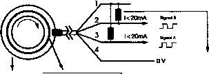

FIGURE 28.16 Connection diagram for SKF sensor bearings.

current position 0 at current time t. The angular difference Oi - Oq can be expressed as An(2n/N), where An is the quantity of pulses counted during the time period At = tl - tQ, and N represents the sensor resolution. Since the output signals are discrete pulses (digital signals or they are transformed to analog ones), in a drive system it is possible to estimate the following four quantities:

1. real-time estimation of the position 0 = 0q-h An(2n/N) if it is assumed that the initial position is known and estimated by additional measures

2. real-time estimation of the angular speed со = d9/dt

3. detection of the speed direction (by using signals A and B)

4. real-time estimation of the acceleration г = dco/dt.

These functions can be performed depending on a customer-specific (motor-specific) interface between the sensor and drive or control systems.

The SKF sensor bearings can replace certain traditional incremental position transducers and can be manufactured at considerably lower cost. Their design is physically robust and withstands the vibrations and higher temperatures in modern drives containing electrical motors with rising power densities and working temperatures. They are also capable of operation in electromagnetically noisy environments.

For illustration purposes, some results are shown in Fig. 28.17 for a DSP-controlled high-performance encoderless induction motor drive employing an SKF sensor bearing. The drive is an encoderless voltage-source inverter-fed DTC induction motor drive using a special torque ripple minimization scheme [40, 41] and employing an SKF sensor bearing (6208). The motor is a 2.2 kW three-phase cage induction motor. It should be noted that the new and simple torque ripple minimization scheme has been implemented since it is known that conventional DTC drives exhibit unwanted torque ripples. This control scheme also contains a mathematical or Al-based model, which utilizes the motor speed, which is

obtained by using the SKF sensor bearing. The results are shown for the reversal of the drive. To iUustrate the fact that the encoderless drive behaves simUarly to the drive with a conventional speed transducer (tachometer). Fig. 28.17 also shows the results obtained when the SKF sensor bearing was not used. As expected, it can be seen that there is very good agreement between the two results.

It can be seen from Fig. 28.17 that the motor can pass through zero speed and the speed obtained by the SKF sensor bearing is almost identical to the speed obtained by the conventional encoder. It is important to note that the induction motor can cross the zero speed safely during reversal. It can be seen that, when the new DTC scheme using the torque ripple minimization technique is used, it is possible to obtain a very attractive total drive solution by using an SKF sensor bearing. To obtain satisfactory low-speed performance, the output signals of the SKF sensor bearing have been processed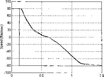

Time (sec)

FIGURE 28.17 Experimental results for a DSP controlled high-performance DTC induction motor drive using an SKF sensor bearing: reversal.

(using a simple and cost-effective artificial-intelligence-based technique) which has increased the resolution.

It has been shown that the SKF sensor bearing can provide information on the rotor speed, acceleration and rotor position of electrical motors. However, this information can also be used for condition monitoring and diagnostic purposes. There are a very large number of possible applications of the SKF sensor bearings, e.g. in electric vehicles, servo drives, etc. The SKF sensor bearings offer a simple, cost-effective, user-friendly solution for motion control purposes. In the future, the sensing function of the bearing can be modified and extended to achieve total customer-specific multifunction micro systems built into smart bearings.

28.3 Motion Control DSPS by Texas Instruments

Various vector and DTC drives have been described above. These can be implemented by using DSPs. For most of these drives it is very suitable to use the new family of Texas Instruments DSP controllers, the TMS320C24x family. This includes six different members based on the 320C2Xlp providing 20 MIPS performance. The 320C24x products support power switching device commutation, command generation, control algorithm processing, data communication and system monitoring functions. All the members offer an ideal single chip solution for digital motor control applications. They include program memory flash or ROM, RAM for the data memory. Event Manager (EV) for generating pulse width modulation signals, A/D converters, UART and CAN controllers.

The TMS320F240 is suitable for an application requiring a large amount of memory on chip, it includes 16Kword of flash, two 10-bit A/D converters, an EV including 3 timers, a serial port interface for an easy connection with other peripherals, an UART, a 16 bit data and address bus for connecting external memory and peripherals.

The TMS320C240 is the ROM based version of the TMS320F240 and is ideal for large volume applications. The EV module is used for operations particularly useful for digital motion control applications. The EV module generates outputs and acquires input signals with a minimum CPU load. Up to 4 input captures and 12 output PWMs are available. The A/D converter module has two 10 bit, 10 ns converters for a total of 16 input channels. Two sample-and-holds allow parallel and simultaneous sampling and conversion. Conversion starts by external signal transition, software instruction or EV event. The reference voltage of the A/D module is 0-5 V: this can be supplied either internally or externally. The device also includes a watchdog timer and a Real Time Interrupt (RTI) module.

The TMS320F241 and TMS320C241 are Skword versions (flash and ROM). They include a new 10bit A/D converter.

which can process the conversion of a signal in less than 850 ns. They are also the first DSPs to contain a CAN controller on chip, which make them ideal for automotive and numerous industrial applications, which require fast and secure communication in noisy environments.

The TMS320C242 is a 4 К ROM based device designed for all motor control applications in the consumer area. The 4 К ROM program memory is satisfactory to include a complete sensorless software which, e.g., will control optimally in space vector mode the speed of an induction motor in a washing machine.

References

1. Baader, U., Depenbrock, M., and Gierse, G. (1992). Direct self control (DSC) of inverter-fed induction machine: a basis for speed control without speed measurement. IEEE Transactions on Ind. Applications IA-28, 581-588.

2. Beierke, S., Vas, R, Simor, В., and Stronach, A. F. (1997). DSP-controlled sensorless ac vector drives using the extended Kalman filter. Power Conversion Intelligent Motion Conference, Numb erg 31-42.

3. Blaschke, P. et al. (1995). Pieldorientirung der geberlosen Drehfeld-maschine. ETZ, 21, pp. 14-23.

4. Blaschke, P., Van der Burgt, J., and Vandenput, A. (1996). Sensorless direct field orientation at zero flux frequency. IEEE IAS Meeting pp. 1/189-1/196.

5. Boldea, L. and Nasar, S. A. (1988). Torque vector control (TVC) - a class of fast and robust torque-speed and position digital controllers for electric drives. Electric Machines and Power Systems 15, 135-147.

6. Bose, B. K. and Simoes, M. G. (1995). Speed sensorless hybrid vector controlled induction motor drive. IEEE IAS Meeting pp. 137-143.

7. Damiano, A., Vas, P., Marongiu, I., and Stronach, A. P. (1997). Comparison of speed sensorless DTC drives. Power Conversion Intelligent Motion Conference, Nurnberg pp. 1-12.

8. Degner, M. W. and Lorenz, R. D (1997). Using multiple sahencies for the estimation of flux, position and velocity in ac machines. IEEE IAS Meeting pp. 760-767.

9. Depenbrock, M. (1985). Direkte Selbstregelung (DSR) fur hochdy-namische Drehfeldantriebe mit Stromrichterschaltung. ETZ A, 7, 211-218.

10. Depenbrock, M. (1988). Direct Self-Control (DSC) of inverter-fed induction machine. IEEE Transactions on Power Electronics 3, 420-429.

11. Depenbrock, M., Hoffman, P., and Koch, S. (1997). Speed sensorless high-performance control for traction drives. European Power Electronics Conference 97, Trondheim pp. 1.418-1.423

12. Du, Т., Vas, P. and Stronach, P. (1995). Design and application of extended observers for joint state and parameter estimation in high-performance ac drives. lEE Proc. Pt. В 142, 71-78.

13. Perrah, A., Bradley, K. J., and Asher, G. M. (1992). Sensorless speed detection of inverter fed induction motors using rotor slot harmonics and fast Fourier transforms. IEEE PES Meeting pp. 279-286.

14. Ha, J. I. and Sul, S. K. (1999). Sensorless field orientation control of an induction machine by high-frequency signal injection. IEEE Transactions on Ind. Applications IA-35, 45-51.

15. Habetler, T. G. and Divan, D. M. (1991). Control strategies for direct torque control using discrete pulse modulation. IEEE Transactions on Ind. Applications 27, 893-901.

16. Jansen, P. L. and Lorenz, R. D. (1995). Transducerless field orientation concepts employing saturation induced saliency in induction machines. IEEE IAS Meeting pp. 174-181.

17. Jiang, J. and Holtz, J. (1998). Accurate estimation of rotor position and speed of induction motors near standstill. IEEE Int Conference on Power Electronics and Drive Systems, Singapore pp. 1-5.

18. Jonsson, R. (1978). NFO drives report, Lund, Sweden.

19. Jonsson, R. and Leonhard, W. (1995). Control of an induction motor without a mechanical sensor, based on the principle of natural field orientation. IPEC, Yokohama pp. 298-303.

20. Kubota, H., Matsuse, K., and Nakano, T. (1990). New adaptive flux observer for induction motor drives. IEEE lECON pp. 921-926.

21. Lagerquist, R. and Boldea, I. (1994). Sensorless control of the synchronous reluctance motor. IEEE Transactions on Ind. Applications IA-30 673-681.

22. Niemela, M (2000). Position sensorless electrically excitated synchronous motor drive for industrial use based on direct flux linkage and torque control. In press.

23. Noguchi, T. and Takahashi, I. (1984). Quick torque response control of an induction motor using a new concept. lEEJ Tech. Meeting on Rotating Machines, paper RM84-76, pp. 61-70.

24. Pyrhonen, J., Pyrhonen, A., Niemela, M., and Luukko, J (1999). A direct-torque-controUed synchronous motor drive concept for dynamically demanding applications. EPE99, Lausanne, paper 215.

25. Sato, I., Kubota, H., and Matsuse, K. (2000). Zero frequency operation for sensorless vector controlled induction machines using extended Kalman filter. IPEC, Tokyo.

26. Schauder, C. (1992). Adaptive speed identification for vector control of induction motors without rotational transducers, IEEE Transactions on Ind. Applications IA-28, 1054-1061.

27. Schroedl, M. (1994). Sensorless control of permanent magnet synchronous motors. Electric Machines and Power Systems 22, 173-185.

28. Takahashi, I. and Noguchi, T. (1985). A new quick response and high efficiency control strategy of an induction motor. IEEE IAS Meeting pp. 496-502.

29. Takahashi, I. and Ohmori, Y. (1989). High performance direct torque control of an induction machine. IEEE Transactions on Ind. Applications IA-25, 257-264.

30. Texas Instruments (1998). TMS320C24x Manual.

31. Tiitinen, P. (1996). The next generation motor control method, DTC, direct torque control. PEDES, pp. 37-43.

32. Vas, P. (1990). Vector Control of ac Machines. Monographs in Electrical and Electronic Engineering Series 22, Oxford University Press, Oxford.

33. Vas, P. (1992). Electrical Machines and Drives: A Space-vector Theory Approach. Monographs in Electrical and Electronic Engineering Series 25, Oxford University Press, Oxford.

34. Vas, P. (1993). Parameter Estimation, Condition Monitoring and Diagnosis of Electrical Machines. Monographs in Electrical and Electronic Engineering Series 27, Oxford University Press, Oxford.

35. Vas, P. (1998). Sensorless Vector and Direct Torque Control. Monographs in Electrical and Electronic Engineering Series 42, Oxford University Press, Oxford.

36. Vas, P. (1999). Artificial-Intelligence-Based Electrical Machines and Drives: Application of Euzzy, Neural, Fuzzy-Neural and Genetic-Algorithm-Based Techniques. Monographs in Electrical and Electronic Engineering Series 45, Oxford University Press, Oxford.

37. Vas, P. and Alakula, M. (1990). Field-oriented control of saturated induction machines. IEEE Transactions on Energy Conversion ec-5, 218-224.

38. Vas, P., Drury, W., and Stronach, A. F. (1996). Recent developments in artificial intelligence-based drives. A review, PCIM, Nurnberg, pp. 59-71.

39. Vas, R, Duits, J., Holweg, E., Rashed, M., and Joukhadar, A. K. M. (2000). Encoderless motion control systems using smart SKF sensor bearings. ICEM, Helsinki.

40. Vas, R, Message, O., Paweletz, O., and Rashed, M. (1999). Multipurpose bearing provides low-cost speed measurement, SKF sensor bearings in encoderless variable-speed electrical drives. AMDC /7/8, 16-18.

41. Vas, R, Stronach, A. R, Rashed, M., Zordan, M., and Chew, B. C. (1999). DSP implementation of sensorless DTC induction motor and p.m. synchronous motor drives with minimized torque ripples. European Power Electronics Conference (EPE99), Lausanne paper 32.

42. Yong, S.I., Choi, J. W., and Sul, S. K. (1994). Sensorless vector control of the induction machine using high frequency current injection. IEEE IAS Meeting, pp. 503-508.

43. Vas, R, Rashed, M., Stronach, A. R, Joukhadar, A. K. M., Ng, C. H., Duits, J., Holweg, E. G. M. (2001). Sensorless drives, state-of-the-art. Power Conversion Intelligent Motion 2001, Nurnberg (invited keynote paper).

44. Vas, R Rashed, M., Joukhadar, A. K. M., Ng, C. H. (2001). Implementation of sensorless induction and permanent magnet synchronous motor drives using natural field orientation. Power Conversion Intelligent Motion 2001, Nurnberg.

Artificial-Intelligence-Based Drives

Professor Peter Vas, Ph.D.

Intelligent Motion Control Group, University of Aberdeen, Aberdeen AB24 SUE, UK

29.1 29.2

29.3 29.4

29.5

General Aspects of the Application of AI-Based Techniques....................... 769

AI-Based Techniques........................................................................... 770

29.2.1 Artificial Neural Networks (ANNs) 29.2.2 Fuzzy Logic Systems (FLSs) 29.2.3 Fuzzy-Neural, Neural-Fuzzy Systems 29.2.4 Genetic Algorithms (GAs)

AI Applications in Electrical Machines and Drives................................... 773

Industrial Applications of AI in Drives by FLitachi, Yaskawa, Texas

Instruments and SGS Thomson............................................................ 774

29.4.1 Hitachi Drive 29.4.2 Yaskawa Drive

Application of Neural-Network-Based Speed Estimators........................... 774

References......................................................................................... 776

29.1 General Aspects of the Application of AI-Based Techniques

In the past four decades considerable research has been performed in the field of artificial inteUigence (fuzzy logic, neural networks, fuzzy-neural networks, genetic algorithms, etc.), which has resulted in many industrial applications. Recent trends and advances in this field have stimulated the development of various artificial-intelhgence-based systems for electrical machine and drive applications. This can also be visualized by the rapidly increasing number of related pubhcations by academics working in the drives field. At present two industrial variable-speed electrical drives incorporate some form of artificial inteUigence (AI). FLowever, the only comprehensive treatment of these techniques for electrical machine and drive apphcations has been presented in a major textbook [20]. This covers the details of Al-based machine design, control, parameter and state estimation (e.g. speed, position, flux, torque, etc., estimation), condition monitoring and diagnosis, simulation (steady state and transient), various firing schemes, etc., for dc drives, induction motor drives, synchronous motor drives (e.g. pm motor drives), switched reluctance motor drives, scalar, vector and DTC drives. In the next few sections, various aspects of Al-based drives are discussed briefly.

Table 29.1 summarizes some of the main advantages offered by the application of artificial inteUigence-based systems (controllers, estimators).

In classical control systems, knowledge of the controUed system (plant) is required in the form of a set of algebraic and differential equations, which analytically relate inputs and outputs. FLowever, these mathematical models are often complex, rely on many assumptions, may contain parameters which are difficult to measure or may change significantly during operation, and sometimes such mathematical models cannot be determined. Furthermore, classical control theory suffers from some limitations due to the nature of the controUed system (linearity, time invariance, etc.). These problems can be overcome by using Al-based control techniques, and these techniques can be used even when the analytical models are not known, and they can be less sensitive to parameter variation (more robust) than classical control systems.

To iUustrate that Al-based techniques have an enormous market potential. Table 29.2 shows the rapidly expanding market of fuzzy logic applications. It can be seen that, in contrast to 1989, where the world market for fuzzy logic applications was only $5 miUion, in 1995 the combined European, Japanese and USA market was $3.8 biUion and it is estimated that by the end of 2000, this wiU increase to $18 biUion, which is 26 times the value of the estimated world market for classical PID controUers.

TABLE 29.1 Main advantages of using Al-based controllers and estimators

Their design does not require a mathematical model of the plant.

They can lead to improved performance (when properly tuned).

They can be designed exclusively on the basis of linguistic information available from experts or by using clustering or other techniques.

They may require less tuning effort than conventional controUers.

They may be designed on the basis of response data in the absence of the necessary expert knowledge.

They may be designed using a combination of linguistic and response-based information.

They can lead to extremely good generahzations (give good estimates when some new unknown input data are used) and thus be independent of particular characteristics of the system (e.g. electrical drive).

They can be easily made adaptive by the incorporation of new data or information as it becomes available.

They may provide solutions to control problems which are intractable by conventional methods.

They exhibit good noise rejection properties.

They are inexpensive to implement, especially if minimum configuration is used.

They are easy to extend and to modify.

A brief overview is now given on the various Al-based techniques.

29.2.1 Artificial Neural Networks (ANNs)

ANNs are universal function approximators and are capable of closely approximating complex mappings, which can be extended to include the modelling of complex, nonhnear systems [20]. In an ANN, there are artificial neurons interconnected via weights. A classical artificial neuron outputs the weighted sum of its inputs and applies a nonlinear activation function (e.g. a sigmoid) on this weighted sum. Thus, if a general, simple static artificial ith neuron has n inputs, and these are Xj, ..., and it outputs a scalar quantity, and the connection weights between the ith neuron and the inputs are Wii, w2,..., then the neuron output is obtained as Yi = fi(J2 Щ]] + i)- this expression / is the activation function of the ith neuron (e.g a sigmoid function), the summation is performed from 1 to n, and is a constant (which is called the bias of the activation function). In an ANN there are various layers, and for example, in a multilayer feedforward ANN, which is the most frequently used ANN,

there are several layers (e.g. an input layer, two hidden layers, an output layer), and each layer contains neurons. Such an ANN is shown in Fig. 29.1. In a multilayer feedforward ANN the neurons in a layer are connected to the neurons of the next layer (via the weights).

Unlike some other types of models, an ANN model can be formed directly by using the input/output data of the unknown system, without the need for any prior model structure. It is very important to note that, in contrast to linear theories, a general ANN model is not assumed to be linear. A supervised neural network can learn the non-linear input-output function of a system in the learning phase (training phase) by observing a set of input-output examples (training set). In the apphcation stage, the trained ANN computes the outputs from the corresponding inputs. The learning phase can also be performed online in realtime and it is possible to perform both the learning and apphcations stages simultaneously (specialized learning). In this case it is possible to adapt the control law to different operating conditions since training is performed onhne.

One of the most widely used supervised ANNs uses the so-called backpropagation algorithm. In the training phase, the inputs and outputs of the ANN are used to obtain the ANN architecture (e.g. weights, if the number of layers, number of nodes and biases and activation functions are fixed) by back-propagating the error (which is the difference between desired output and actual output). This technique is based on a steepest descent approach to minimize the prediction error with respect to the connection weights in the neural network, i.e. the gradient formula is used for weight adjustement: Wji(k + 1) = Wji(k) + Awjp where Awj is the change made to the weights, and it is proportional to the negative rate of change of the error with respect to the weights (Awji -dE/dwp where E is the total network error). The training stage is easy to understand: if the multilayer feedforward neural network (e.g. a four-layer network shown in Fig. 29.1 containing an input layer with three input signals.

two hidden layers and an output layer with two output signals) gives incorrect outputs, the weights are corrected so that the error is reduced and future network responses wiU be more accurate. The initial weights are obtained randomly, and these are then changed by using the backpropagation algorithm. Once the training stage is over, the architecture of the ANN is fixed and in the application stage new inputs are apphed and the associated outputs are computed. Although the backpropagation algorithm is simple, it is a disadvantage that the convergence time of the learning algorithm can be slow and the learning speed is a crucial factor for training a neural network, especially for a large neural network with large training data sets. Much research has been done to improve the learning speed of the backpropagation algorithm, but some of these increase the complexity of the neural network. It is also possible to enhance the backpropagation learning by using fuzzy concepts. It is another disadvantage of the back-propagation algorithm that the minimization of the error does not guarantee that a global minimum wiU be obtained, and instead a local minimum can be reached, but the local minima can also be avoided by using genetic algorithm-assisted weight selection.

29.2.2 Fuzzy Logic Systems (FLSs)

Fuzzy logic systems (FLSs) are also universal function approximators. FLowever, a fuzzy logic system is an expert system, where the heart of a fuzzy logic system (FLS) is a hnguistic rule-base, which can be interpreted as the rules of a single overall expert, or as the rules of subexperts and there is a mechanism (inference mechanism) where all the rules are considered in an appropriate manner to generate the output(s) [20]. These rules may directly originate from experts, but if the experts are not available, they can also be obtained by the appropriate processing (e.g. clustering) of available input/output data. Again it is important to note that the system can be nonlinear, and nonhnearity is incorporated into the fuzzy logic system.

A nonlinear function can also be approximated by using a finite set of expert (fuzzy) rules. These rules form a rule-base and an individual rule can be considered as a rule of a subexpert (local expert). The whole set of rules can be considered as the rules of a main-expert (global expert). A fuzzy function approximator with finite number of rules can approximate any continuous function on a compact domain to any degree of accuracy. Each rule defines a bounded region of the input-output space. The fuzzy approximator approx-

imates a function, which covers its curve with rule regions and adds or averages regions that overlap. In general, the number of rules required (to cover the curve to be approximated) grows exponentially with the number of input and output variables. Lone optimal rule regions cover the extrema of the approximand and offer one way to deal with the rule expansion. Learning has the effect of moving and shaping the rule regions. The best learning techniques rapidly find and cover the extrema and bumps in the curve to be approximated and then move rule regions between the extrema as the rule budget allows.

A rule-base contains the whole set of fuzzy rules for a specific apphcation, i.e. for a nonlinear function approximation. The fuzzy rules have an if-then structure and involve linguistic values for the input and output variables. In general, a fuzzy rule can take the following form:

If Xl is A and X2 is В then у is C.

In the rules A, В and С represent fuzzy sets, e.g. A can correspond to the smaU fuzzy set of x, В can correspond to the medium fuzzy set of X2 and С can correspond to the large fuzzy set of y. For example, in a fuzzy logic speed controller with two inputs, input Xi input is the error, input X2 is the change of the error, and A corresponds to the fuzzy set of errors which belongs to the smaU errors, В corresponds to the fuzzy set of change of errors which belongs to the medium change of errors, etc.

Figure 29.2 shows the schematic of a Mamdani-type fuzzy-logic-based system (function approximator) [20]. Since the rule-base contains hnguistic rules, and since the input data are crisp data, they have to be transformed into linguistic values (by using fuzzification and for this purpose membership functions are used). This is why in general, the fuzzy logic approximator contains the Transformation 1 block, which performs fuzzification. Similarly, on the output of the fuzzy approximator a crisp output value must be present, and this is obtained by transforming the linguistic outputs into crisp output via the Transformation 2 block (defuzzifier). There are many types of defuzzifiers, e.g. centre of gravity defuzzifier, centroid defuzzifier, etc. In the second block, the inference operation (decision making) is performed, i.e. by using the rule-base and knowledge base (which contains knowledge of the system), the inference operation calculates the corresponding fuzzy (linguistic) output(s) from the input(s) (there are many types of inference engines, e.g. the one using the max-min method, the max-dot product, etc. [20]). In a realtime

Fuzzy function approximator

У=т

FIGURE 29.2 Mamdani-type fuzzy-logic-based system (function approximator).

implementation of a fuzzy logic system it is a very important goal to approximate a given function accurately by a minimum number of rules (since this leads to less computation time and allows the use of a cheaper DSP).

There are various types of fuzzy logic systems, but the three main types are the Mamdani, the Sugeno and the Tsukamoto fuzzy logic systems [20]. The Sugeno type has been extensively used in Japan, and in contrast to the Mamdani-type FLS, it does not contain a defuzzifier.

29.2.3 Fuzzy-Neural, Neural-Fuzzy Systems

It is possible to combine neural networks with fuzzy logic systems, and the arising integrated system can be a fuzzy-neural or neural-fuzzy system [20], which is also a nonlinear system. In contrast to a purely neural multilayer system (multilayer ANN-based system), where the number of hidden layers and number of hidden nodes (in a hidden layer) are not known a priori (but only after intensive calculations), it is an advantage of the fuzzy-neural and neural-fuzzy systems that they already incorporate some form of expertise and the architecture of the systems is well-defined a priori. Thus the number of hidden layers is exactly known and also the number of hidden nodes is also known.

Since both fuzzy and neural systems are universal function approximators, their combination, the hybrid fuzzy-neural system (or neural-fuzzy system) is also a universal function approximator.

The major drawback of conventional neural networks is that, although they can be used to approximate any nonlinear mapping, in general they can be viewed as black boxes, without providing general explanations. Thus although the inherent black box approach provides the correct solutions, it does not provide heuristic interpretation of the solution. However, engineers prefer accurate function approximation as well as the heuristic knowledge behind this process. Fuzzy logic can be conveniently used to provide heuristic reasoning: the behavior of a fuzzy logic system can be easily understood, due to its logical structure and simple inference mechanism. Furthermore, in an artificial neural network, the required number of hidden layers and the number of hidden nodes is not known a priori. In contrast to this, in the hybrid system (fuzzy-neural system), the architecture (structure) of the system is known and is decided by fuzzy principles. In a fuzzy-neural network there is no need for a priori information of the membership functions (their number and also their shapes), and for a priori information on the rule-base these can be obtained by the appropriate tuning of the fuzzy-neural network. The state-of-the-art intelligent control is at the level of adaptive fuzzy-neural controllers.

There are various types of fuzzy-neural systems, but the four main types of fuzzy-neural systems are: the Mamdani

type, the Sugeno type, the Tsukamoto type and the Wang type [20].

Similar to conventional ANNs, the training of a fuzzy-neural network can be performed by using the backpropagation algorithm. However, some difficulties may occur in the direct implementation of this, when the activation functions are nondifferentiable, but this problem can also be solved by modifying the original backpropagation algorithm.

29.2.4 Genetic Algorithms (GAs)

Genetic algorithms (GAs) [20], are not function approximation techniques, but they are simple and powerful general-purpose stochastic optimization methods (learning mechanisms), which have been inspired by the Darwinian evolution of a population subject to reproduction, crossover and mutations in a selective environment where the fittest survive. GA combines the artificial survival of the fittest with genetic operators abstracted from nature to form a very robust mechanism that is suitable for a variety of optimization problems.

In mathematical terms the goal of the genetic algorithm is to minimize an objective functions F(S]J, where Sj is the search candidate (optimal solution), which is the kth individual in the population S (where the population is the set of possible solutions). The individuals of the population are expressed in a binary string form (the initial binary strings corresponding to the initially assumed individuals are, e.g., obtained by a random process) and the GA then manipulates these strings by using genetic operators (reproduction, crossover, mutation) to obtain improved solutions (where the fittest individuals survive) until the optimal solution is obtained.

It is one of the main advantages of a GA that it uses stochastic operators instead of deterministic rules to search for a solution. Furthermore, a GA considers many points in the search space simultaneously, not a single point; thus it has a reduced chance of converging to local minima, in which other algorithms might end up. Thus the global optimum of the problem can be approached with higher probability. It follows that, in addition to producing a more global search, it is another attractive feature of GA that it searches for many optimum points in parallel (simultaneous consideration of many points), since the evaluation of each point requires an independent computation. The data processed by the algorithm is a set (population) of binary strings (chromosomes), which represent multiple points in the search space. Due their robustness, speed, efficiency and flexibility GAs have so far been used in various engineering and business problems.

The input data processed by the genetic algorithm is used to create an initial population (set of possible solutions) either randomly or heuristically. The individuals in this population carry chromosomes, which are the variables. During each