iteration step of the algorithm, which is caUed a generation, structures in the current population are evaluated and new generations are formed. The structures of the population are chosen by a randomized selection process, which ensures that the expected number of times a structure is chosen is approximately equal to that structures performance (fitness) relative to the rest of the population. The less fit individuals in the population die and, in order to search other points in the space, some variations are introduced into the new population by using ideahsed genetic recombination (transitional) operators (e.g. crossover, mutation, etc.). Thus the fittest individuals (solutions) are bred, i.e. two individuals are mated (crossover) and the offspring of the mated pair receives some characteristics of the parents. Fit individuals carry on mating, and some of them mutate; thus the population undergoes various generation changes. After many generations, a population (solution) emerges, where the individuals will solve the problem weU.

It can be seen that, in the genetic algorithm, it is necessary to use a fitness function and its selection is crucial. It must reflect the controUers ability to reach the setpoint from a number of initial condition cases. It is very important to note that GAs consider many points in the search space, and thus have a reduced chance of converging to local minima. Furthermore, the simultaneous consideration of many points makes them adaptable to parallel processors since the evaluation of each point requires an independent computation.

There are various possibilities for the application of GAs:

In GA-assisted multilayer artificial neural networks, GAs can be used to optimize the size of a hidden layer and also the weights (strength of connections connecting the artificial neurons of the ANN). This is justified by the foUowing two factors:

- it aUows one to avoid local optima and provides near-global optimization solutions

- it is easy to implement.

Fiowever, it must also be considered that too many hidden neurons (neurons in the hidden layer) decrease the generalization capability of the network and also imply a long learning phase. On the other hand, a network with too few neurons can be unable to learn the given function with the desired precision. Thus there is an intermediate number of hidden neurons required to avoid the problems mentioned above.

GAs can also be used to obtain the membership functions and the rule-base in a fuzzy-logic controUer.

In GA-based controUers, genetic algorithms are used to learn the controUer structure from scratch and also to tune the controller parameters.

GAs can be used to estimate coefficients (parameters) contained in nonlinear algebraic equations.

For example, it is also possible to obtain the electrical parameters of an electrical machine by using GA-based parameter estimation. For this purpose, the initial parameter values are generated randomly, and these form the initial individuals of the population. The GA is then used to obtain the individuals of the final population (final values of the machine parameters) [20].

Finally it should be noted that it is possible to implement Al-based self-repairing, self-contructing controllers and estimators, e.g. in variable-speed, high-performance, sensorless drives by using GA. For this purpose an FPGA (Field Programmable Gate Array) can be used [20].

29.3 AI Applications in Electrical Machines and Drives

In the literature most publications on the application of artificial inteUigence (AI) in electrical drives discuss fuzzy-logic-based, or seldom neural-network-based, speed or position controUer applications, where an existing PI or PID controUer is simply replaced by an Al-based controUer. Although this is an important application, and the Al-based controUers can lead to improved performance, enhanced tuning and adaptive capabUities, there are further possibUities for a much wider range of Al-based apphcations in variable-speed ac and dc drives. Some of these are also shown in Table 29.3 [20].

AU of these applications are discussed in detail in [20].

TABLE 29.3 Applications of AI in variable-speed drives (ac and dc drives) including the modelling of drives and machine design

Replacement of classical speed, position and other controllers by Al-based controllers. New and combined control structures in various drives including high-performance ac drives: vector and direct torque control (DTC) drives, energy efficient drives, new Al-based universal drives, new Al-based electronic motors .

Al-based new firing signal generation schemes, (e.g. PWM schemes), new switching vector schemes (e.g. in DTC drives).

Al-based compensation of non-linear effects in discontinuous operation.

Al-based parameter estimators, self-commissioning systems.

Al-based speed and position estimators, flux and torque estimators, virtual sensors (e.g. virtual vibration sensor).

Al-based condition monitoring, diagnosis.

Al-based improved observers (e.g. improved Kalman filter, improved extended Kalman filter).

Al-based harmonic estimators (e.g. harmonic identifiers utilizing space vector loci).

Al-based efficiency optimizers.

Al-based machine design.

Al-based steady-state and transient models (to replace conventional mathematical models).

Al-based self-rep airing and self-constructing controllers, schemes.

29.4 Industrial Applications of AI in Drives by Hitachi, Yaskawa, Texas Instruments and SGS Thomson

As mentioned earlier, at present there are two large electrical drive manufacturers, who incorporate artificial intelligence into their drives, Hitachi and Yaskawa. In addition to these it should be noted that Texas Instruments (TI) has developed a fuzzy-controlled induction motor drive using the TMS320C30 DSP. The main conclusion obtained by TI agrees with that of the present author obtained from various fuzzy control implementations: the development time of the fuzzy-controlled drive is significantly less than the corresponding development time of a drive using classical controllers. SGS Thomson has also developed various fuzzy-neural controlled drives.

29.4.1 Hitachi Drive

According to Hitachi, the J300 series IGBT inverter based sensorless vector drive is the first industrial drive which incorporates fuzzy logic [20]. According to Hitachi the intelligent inverter takes into account the characteristics of both the motor and the system and the torque computation software ensures accurate torque control throughout the entire frequency range, even with general purpose motors . Some of the main characteristics are shown in Table 29.4.

Fuzzy logic control is used in the Hitachi drive for the calculation of optimum acceleration and deceleration times, and according to Hitachi there is fuzzy logic control of both the motor current and ramp rate during drive acceleration and deceleration . The calculations are based on motor load and braking requirements (thus eliminating the need for adjustments using trial and error). The fuzzy logic acceleration/deceleration function sets acceleration and deceleration factors and speed according to fuzzy rules which use the distance up to the overload limit (or other limits), and also the start-up gradient of motor current and voltage. According to Hitachi, the main advantages of using fuzzy logic control are: when conventional, simple current hmit control is used, the inverter ramps are stepped and the drive can often trip out, specially during deceleration. However, when fuzzy logic

TABLE 29.4 Main characteristics of Hitachi J300 series induction motor drive [20]

High starting torque of 150% or more at 1 Hz

100% continuous operating torque within a 3:1 speed range

(20-60 Hz/16-50 Hz) without motor derating Speed regulation ratio as smaU as ±1% High-speed microcomputer and built-in DSP The improved response speed characteristic is effective in preventing

slip-down in hfting equipment apphcations Torque response speed of approximately 0.1 s can be achieved Fuzzy logic control

control is used, the ramps are very smooth and nuisance tripping is eliminated . Possible applications of the drive include fan or pump applications where constant acceleration or deceleration times or accurate position control are not required, but optimization of the speed ramp dependent on the load conditions is required. By using fuzzy control, the most efficient ramp time can be guaranteed, whilst also ensuring trip free running.

29.4.2 Yaskawa Drive

Fenner Power Transmission UK has teamed up with Yaskawa, to market the Yaskawa intelligent induction motor drive range. Top of the range is the VS-616G5 so-called True Flux Vector Inverter . The VS-616G5 is a general purpose inverter which also contains flux vector control that directly controls the currents (or torque) in an induction motor. According to Yaskawa it contains a magnetic flux observer with intelligent neuro control , which ensures direct torque control and this enables the VS-G16G5 to surpass the performance of comparable dc motor controllers and provides a less expensive alternative [20].

29.5 Application of Neural-Network-Based Speed Estimators

In Chapter 20 various speed and position sensorless ac motor drive schemes are discussed. However, in addition to using mathematical-model-based estimators, it is also possible to use, e.g., ANN-based speed estimators in ac and dc drives. Such drives have been successfully implemented by the author [20]. Some aspects of an ANN-based speed sensorless medium-performance induction motor drive are now discussed. Medium performance induction motor drives represent a large and important share of the induction motor drives market. Rehable, stable, and simple scalar induction motor drives are continuously under development by various manufacturers. Scalar drives are widely used in various industrial fields. The drive to be considered here is a speed-sensorless scalar controlled induction motor drive, which contains a minimum configuration ANN-based speed estimator. For this purpose only two stator currents are monitored. The schematic of the drive scheme is shown in Fig. 29.3.

In Fig. 29.3 the speed controller is a classical PI controller, but Al-based controllers can also be used. The speed controller generates the reference angular shp frequency (cOgij-ef)- The drive scheme contains a frequency-to-voltage conversion block, a block where the reference stator voltages are generated, a transformation block, a PWM inverter which supplies the motor and a speed estimator ANN. The inputs to the PWM modulator are the stator reference voltages. The full control system (which also includes the speed estimator ANN), has been implemented by using the Texas Instruments

Ш

rref

slref %

converter

Transformation

sDref

PWM Inverter

Transformation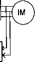

FIGURE 29.3 Sensorless scalar induction motor drive scheme using an ANN-based speed estimator.

TMS320C30 DSP. Although for simplicity they are not shown, there are two further inputs to the frequency/voltage converter block: these take account of the stator ohmic voltage drops.

The ANN shown in Fig. 29.3 is a multilayer feedforward backpropagation ANN. It utilizes three input signals: these are the modulus of the stator voltage space vector and two transformed stator currents. The transformed stator currents are obtained by the application of the appropriate transformation from the monitored direct and quadrature axis stator currents in the stationary reference frame, ( 4q)- Various possibilities have been investigated to obtain the most optimal transformation. The feedforward multilayer ANN has three layers: an input layer, a single hidden layer and an output layer. The number of hidden neurons in the hidden layer was obtained by trial and error. Sigmoid activation functions were used in the hidden nodes. The output node is a hnear node, and outputs the angular rotor speed.

It is very important to note that rapid implementation was obtained and the training of the ANN was achieved by using training data obtained by simulation of the complete drive system. The training was performed by using the backpropagation algorithm discussed above. When the trained ANN was implemented, the very first implementation of the sensorless induction motor drive (using the ANN-based speed estimator) worked. The training took only a few minutes on a PC and for this purpose 11,000 input-output training data sets were used. Figure 29.4 shows some of the training signals used: the top curve shows the speed training signal and the bottom curve shows the two transformed stator currents.

Although the training of the ANN was performed with data for the unloaded 3 kW induction motor, the speed-sensorless drive also worked weU when the motor was lightly loaded. Fiowever, for operation with high loads, the neural network had to be retrained. The simple minimum configuration speed estimator ANN enabled a very fast implementation.

In Fig. 29.5 there is shown the experimentally obtained speed response to random speed reference changes for the lightly loaded 3 kW motor.

To illustrate the accuracy of the resuhs, in Fig. 29.5 the measured speed is also shown, but it is important to note that this has not been used in the drive scheme. It can be seen that

there is very good agreement between the measured and estimated speeds. It is important to note that the same trained ANN as used for the 3 kW motor was successfully used in the scalar drive employing a 2.2 kW induction motor. Some experimental results for the drive incorporating this motor are also presented in Fig. 29.6, where the motor reverses from 60 rad/s to -60 rad/s. Fiowever, in Fig. 29.6, results are also shown when a recursive ANN is used. The inputs to the recursive ANN are the same signals as for the feedforward multilayer ANN, but there is an extra input signal, which is the past sampled value of the rotor speed.

There are three curves shown in Fig. 29.6. The top (black) curve shows the measured value of the rotor speed, the curve in the middle (blue curve) corresponds to the estimated speed when the recursive ANN is used and the bottom (red) curve corresponds to the speed estimated by the feedforward multilayer ANN. It can be seen that the drive with the recursive ANN-based speed estimator gives better results than the one with the multilayer feedforward ANN.

Various other types of ANN-based speed estimators have also been discussed for induction motors and synchronous motors in [20], including Model Reference Adaptive System (MRAS)-based estimators as weU, where the MRAS system (see also Chapter 20) contains an ANN. Work is under progress on various types of sensorless high-performance induction motor and permanent magnet synchronous motor drives, which can also be used at very low (including zero) stator frequencies and under high load conditions. For this purpose Al-based and also other schemes are being developed which do not require extra hardware or modifications to the motor. These include both vector- and direct-torque-controUed drives.

It is believed that, in the future, some of the problems associated with reluctance motor control, e.g. switched reluctance motors (pulsating torque, noise, etc.) can be ehminated by using Al-based controllers. The switched reluctance machine is a highly nonlinear doubly salient machine and its mathematical model is complicated. Fiowever, these properties make this type of machine ideal to be subjected to Al-based control. It is expected that various types of torque-controlled Al-based switched reluctance motor drives wiU also emerge.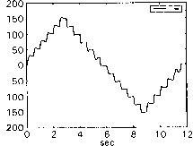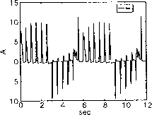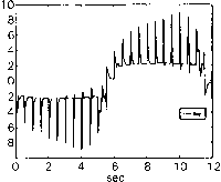

FIGURE 29.4 Training signals for multilayer feedforward ANN-based speed estimator.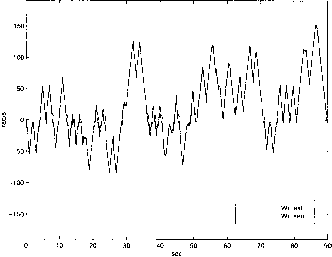

FIGURE 29.5 Experimental results for a sensorless induction motor drive scheme (using a multilayer feedforward ANN-based speed estimator) for random speed reference changes (3kW induction motor).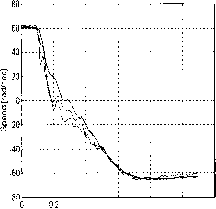

04 0,6 0.8 Time (sec)

FIGURE 29.6 Experimental results for a sensorless induction motor drive with multilayer feedforward ANN and also with recursive ANN-based speed estimator (2.2 kW induction motor).

References

1. Beierke, S., Vas, R, and Stronach, A. R (1997). TMS320 DSP Implementation of fuzzy-neural controUed induction motor drives, European Power Electronics Conference, Trondheim, pp. 2.449-2.453.

2. Cirrincione, M., Rizzo, R., Vitale, G., and Vas, R (1995). Neural networks in motion control: theory, an experimental approach and verification on a test bed. Power Conversion Intelligent Motion Conference, Nurnberg, pp. 131-141.

3. Pilippetti, R, Pranceschini, G., Tassoni, C., and Vas, R (1998). AI techniques in induction machine diagnosis including the speed ripple effect. IEEE Transactions on Energy Conversion 34, 98-108.

4. Grundman, S, Krause, M., and MuUer, V. (1995). Apphcation of fuzzy control for PWM voltage source inverter fed permanent magnet motor. EPE, Seville, pp. 1.524-1.529.

5. Hertz, J., Krogh, A., and Palmer, R. G. (1991). Introduction to the

Theory of Neural Computation. Addison Wesley, Redwood City, CA.

6. Hofinan, W. and Krause, M. (1993). Fuzzy control of ac drives fed by PWM inverters. PCIM, Nurnberg, pp. 123-132.

7. Mamdani, E. H. (1974). Application of fuzzy algorithms for simple dynamic plant. Proc. lEE 111, 1585-1588.

8. Jang, J. G. (1993). ANFIS: adaptive-network-based fuzzy inference system. IEEE Transactions on System, Man and Cybernetics SMC- 23, 665-684.

9. Monti, A., Roda, A., and Vas, P. (1996). A new fuzzy approach to the control of the synchronous reluctance machine. EPE, PEMC, Budapest, pp. 3/106-3/110.

10. Simoes, G. and Bose, B. K., (1995). Neural network based estimation of feedback signals for a vector controlled induction motor drive. IEEE Transactions on Ind. Applications IA-31, 620-629.

11. Stronach, A. F. and Vas, P. (1995). Fuzzy-neural control of variable-speed drives. PCIM, Nurnberg, pp. 117-129.

12. Stronach, A. R, Vas, P., and Neuroth, M. (1997). Implementation of intelligent self-organising controllers in DSP-controlled electromechanical drives. lEE Proc. Pt D 143, 324-330.

13. Sugeno, M. and Kang, G. T. (1988). Structure identification of fuzzy model. Euzzy Sets and Systems 15-33.

14. Vas, P. (1992). Electrical Machines and Drives: A Space-Vector Theory Approach. Monographs in Electrical and Electronic Engineering Series 25, Oxford University Press, Oxford.

15. Vas, P. (1993). Parameter Estimation, Condition Monitoring and Diagnosis of Electrical Machines. Monographs in Electrical and Electronic Engineering Series 27, Oxford University Press, Oxford.

16. Vas, P. (1995). Artificial intelligence applied to variable-speed drives. PCIM Seminar, Nurnberg, pp. 1-149.

17. Vas, P. (1996). Recent trends and development in the field of machines and drives, application of fuzzy, neural and other intelligent techniques. Workshop on AC Motor Drives Technology, IEEE/IAS/PELS, Vicenza, pp. 55-74.

18. Vas, P. (1998). Sensorless Vector and Direct Torque Control. Monographs in Electrical and Electronic Engineering Series 42, Oxford University Press, Oxford.

19. Vas, P. (1998). Speed and position sensorless and artificial-intelligence-based dc and ac drives. PCIM, Nurnberg, pp. 1-198.

20. Vas, P. (1999). Artificial-Intelligence-Based Electrical Machines and Drives: Application of Euzzy, Neural, Fuzzy-Neural and Genetic-

Algorithm-Based Techniques. Monographs in Electrical and Electronic Engineering Series 45, Oxford University Press, Oxford.

21. Vas, P. and Drury, W. (1995). Future trends and developments of electrical machines and drives. PCIM, Nurnberg, pp. 1-28.

22. Vas, P. and Drury, W. (1996). Future developments and trends in electrical machines and variable-speed drives. Energia Elettrica 73, 11-29.

23. Vas, P., Drury, W, and Stronach, A. F. (1996). Recent developments in artificial intelligence-based drives. A review. PCIM, Nurnberg, pp. 59-71.

24. Vas, R, Li, J., Stronach, A. R, and Lees, R (1994). Artificial neural network-based control of electromechanical systems. 4th European Conference on Control, IFF, Coventry, pp. 1065-1070.

25. Vas, R, Stronach, A. R, Neuroth, M., and Du, T. (1995). Fuzzy, pole-placement and PI controller design for high-performance drives. Stockholm Power Tech. 1-6.

26. Vas, R, Stronach, R, Neuroth, M., and Du, T. (1995). A fuzzy controlled speed-sensorless induction motor drive with flux estimators. IFF FMD, Durham, pp. 315-319.

27. Vas, R and Stronach, A. R (1995). DSP-controlled intelligent high performance ac drives. Present and future. Colloquium on Vector Control and Direct Torque Control of Induction Motors. lEE, London, pp. 7/1-7/8.

28. Vas, P. and Stronach, A. F. (1996). Design and application of multiple fuzzy controllers for servo drives. Archiv fur Flektrotechnik 79, 1-12.

29. Vas, P. and Stronach, A. F. (1996). Minimum configuration soft-computing- based DSP controlled drives. PCIM, Nurnberg, pp. 299-315.

30. Vas, P. and Stronach, A. R (1996). Adaptive fuzzy-neural control of high-performance drives. IFF PEVD, Nottingham, pp. 424-429.

31. Vas, P., Stronach, A. R, and Drury, W. (1996). Artificial intelligence in drives. PCIM Europe 8, 152-155.

32. Vas, R, Stronach, A. R, Rashed, M., Zordan, M., and Chew, B. C. (1999). DSP implementation of sensorless DTC induction motor and p.m. synchronous motor drives with minimized torque ripples. European Power Electronics Conference (FPF99), Lausanne paper 32.

33. Wang, Li-Xin (1994). Adaptive Fuzzy Systems and Control. PTR Prentice Hall, Englewood Cliffs, NJ.

34. Zadeh, L. A. (1965). Fuzzy sets. Information Control 8, 338-353.

Fuzzy Logic In Electric Drives

Ahmed Rubaai, Ph.D.

Department of Electrical Engineering Howard University Washington, D.C. 20059

30.1 Introduction...................................................................................... 779

30.2 The Fuzzy Logic Concept..................................................................... 779

30.2.1 The Fuzzy Inference System (FIS) 30.2.2 Fuzzification 30.2.3 The Fuzzy Interence Engine 30.2.4 Defuzzification

30.3 Applications of Fussy Logic to Electric Drives......................................... 784

30.3.1 Fuzzy Logic-Based Microprocessor Controller 30.3.2 Fuzzy Logic-Based Speed Controller 30.3.3 Fuzzy Logic-Based Position Controller

30.4 FLardware System Description............................................................... 788

30.4.1 Experimental Results

30.5 Conclusion........................................................................................ 789

References......................................................................................... 790

30.1 Introduction

Over the years, we have increasingly been on the search to understand the human ability to reason and make decisions, often in the face of only partial knowledge. The ability to generahze from limited experience into areas as yet unencoun-tered is one of the fascinating abilities of the human mind. Traditionally, our attempt to understand the world and its functions has been limited to finding mathematical models or equations for the systems under study. This approach has proven extremely useful, particularly in an age when very fast computers are available to most of us with only a minimum amount of capital outlay. And even when these computers are not fast enough, many researchers can gain access to supercomputers capable of giving numerical solutions to multiorder differential equations that are capable of describing most of the industrial processes.

This analytical enlightenment, however, has come at the cost of realizing just how complex the world is. At this point, we have come to realize that, no matter how simple the system is, we can never hope to model it completely. So instead, we select suitable approximations that give us answers that we think are sufficiently precise. Because our models are incomplete, we are faced with one of the foUowing choices:

1. Use the approximate model and introduce probabU-istic representations to aUow for the possible errors.

2. Seek to develop an increasingly complex model in the hope that we can find one that completely describes the systems while being solvable in real time.

This dilemma has led a few, most notably Zadeh [14], to look at the decision-making process employed by our briUiant minds when confronted with incomplete information. The approach taken in those cases makes allowances for the imprecision caused by incomplete knowledge and actually embracing the imprecision in forming an analytical framework. This approach involved artificial inteUigence using approximate reasoning, or fuzzy logic as it is now commonly known. As a result, artificial inteUigence using fuzzy logic has proven extremely useful in ascribing a logic mechanism to a wide range of topics from economic modeling and prediction to biology analysis to control engineering. In this chapter, an examination of the principles involved in artificial inteUigence using fuzzy logic and its application to electric drives is discussed.

30.2 The Fuzzy Logic Concept

Fuzzy logic arose from a desire to incorporate logical reasoning and the intuitive decision making of an expert operator into an automated system [14]. The aim is to make decisions based on a number of learned or predefined rules, rather than numerical calculations. Fuzzy logic incorporates a rule-base structure in attempting to make decisions [2,3,4,5,14]. FLowever, before the rule-base can be used, the input data should be represented in such a way as to retain meaning, while StiU aUowing for manipulation. Fuzzy logic is an aggregation of rules, based on the input state variables condition with a corresponding desired output. A mechanism must exist

to decide on which output, or combination of different outputs, will be used since each rule could conceivably result in a different output action.

Fuzzy logic can be viewed as an alternative form of input/output mapping. Consider the input premise, x, and a particular qualification of the input x represented by A. Additionally, the corresponding output, y, can be qualified by expression Q. Thus, a fuzzy logic representation of the relationship between the input x and the output у could be described by the following:

R: IF xisAi THEN у is Cl

R2: IF xisA2 THEN у is c2 (30.1)

R: IF X is A THEN у is C

where x is the input (state variable), у is the output of the system, Al are the different fuzzy variables used to classify the input X and Q are the different fuzzy variables used to classify the output y.

The fuzzy rule representation is linguistically based [3,14]. Thus, the input x is a linguistic variable that corresponds to the state variable under consideration. Furthermore, the elements A are fuzzy variables that describe the input x. Correspondingly, the elements Q are the fuzzy variables used to describe the output y. In fuzzy logic control, the term linguistic variable refers to whatever state variables the system designer is interested in [14]. Linguistic variables that are often used in control applications include Speed, Speed Error, Position, and Derivative of Position Error. The fuzzy variable is perhaps better described as a fuzzy linguistic quahfier. Thus the fuzzy qualifier performs classification (qualification) of the linguistic variables. The fuzzy variables frequently employed include Negative Large, Positive Small and Zero. Several papers in the literature use the term fuzzy set instead of fuzzy variable , however; the concept remains the same. Table 30.1 illustrates the difference between fuzzy variables and linguistic variables.

Once the hnguistic and fuzzy variables have been specified, the complete inference system can be defined. The fuzzy linguistic universe, (7, is defined as the collection of all the fuzzy variables used to describe the linguistic variables [6,7,8], i.e. the set U for a particular system could be comprised of Negative Small (NS), Zero (ZE) and Positive Small (PS). Thus, in this case the set (7is equal to the set of [NS, ZE, PS]. For the system described by Eq. (30.1), the linguistic universe for the input X would be the set = [А^Аз ... А„]. Similarly,

table 30.1 Fuzzy and linguistic variables

Linguistic Variables

Fuzzy Variables (Linguistic Qualifiers)

Speed error Position error Acceleration Derivative of

position error Speed

(SE) (PE) (AC) (DPE)

Negative large Zero

Positive medium Positive very small

(SP) Negative medium small

(NL) (ZE) (PM) (PVS)

(NMS)

the linguistic universe for the output у would be the set l/, = [QQ...C .

30.2.1 The Fuzzy Inference System (FIS)

The basic fuzzy inference system (FIS) can be classified as:

Type 1 Fuzzy Input Fuzzy Output (FIFO) Type 2 Fuzzy Input Crisp Output (FICO)

Type 2 differs from the first in that the crisp output values are predefined and, thus, built into the inference engine of the FIS. In contrast, type 1 produces linguistic outputs. Type 1 is more general than type 2 as it allows redefinition of the response without having to redesign the entire inference engine. One drawback is the additional step required, converting the fuzzy output of the FIS to a crisp output.

Developing a FIS and applying it to a control problem involves several steps:

1. fuzzification

2. fuzzy rule evaluation (fuzzy inference engine)

3. defuzzification.

The total fuzzy inference system is a mechanism that relates the inputs to a specific output or set of outputs. First, the inputs are categorized hnguistically (fuzzification), then the hnguistic inputs are related to outputs (fuzzy inference) and, finally, all the different outputs are combined to produce a single output (defuzzification). Figure 30.1 shows a block diagram of the fuzzy inference system.

30.2.2 Fuzzification

Fuzzification is the conversion of crisp numerical values into fuzzy linguistic quantifiers [7,8]. Fuzzification is performed using membership functions. Each membership function evaluates how well the linguistic variable may be described by a particular fuzzy quahfier. In other words, the membership

figure 30.1 Fuzzy inference system.

function derives a number that is representative of the suitability of the hnguistic variable to be classified by the fuzzy variable (set). This suitability is often described as the degree of membership. In order to maintain a relationship to traditional binary logic, the membership values must range from 0 to 1 inclusive. Figure 30.2 shows the mechanism involved in the fuzzification of crisp inputs when multiple input are involved. Since each input has a number of membership functions (one for each fuzzy variable), the outputs of aU the membership functions for a particular crisp numerical input are combined to form a fuzzy vector.

Any number of normalizing expressions can perform fuzzification. Two of the more common functions are the hnear and Gaussian [4]. In both cases there is one parameter, /л, that indicates the midpoint of the region and another, cr, that defines the width of the membership functions. For the hnear function, the width is specified by and the midpoint by l-Similarly for the Gaussian function, the width is specified by (Tq and the midpoint by лq. Equations (30.2(a)) and (30.2(b)) define the linear and Gaussian membership functions, respectively:

Linear function:

ifxe [(l - l) (il + l)] Otherwise

(30.2(a))

Gaussian function: expl -

ut-l

ut-2

M mb r h Fu ct

M mb r h Fu ct

M mb r h Fu ct

Mmbrh Fuct

(30.2(b))

u у V ct r

I-►

Mmbrh Fuct

Mmbrh Fuct ~-

Fu у Vctr F r ut-2

Mmbrh Fuct

M mb r h Fu ct

M mb r h Fu ct

I Fu у Vctr

(7l = 3(7g.

(30.3(a)) (30.3(b))

The relations expressed by Eqs. (30.3(a)) and (30.3(b)) are made because of the characteristics of the Gaussian function. Because a Gaussian membership function may never have a membership value of 0, some appropriate value close to zero must be chosen as the cutoff point. At a distance of 3(Jq from the mean, the Gaussian membership function results in a membership value of 0.05. Thus the width of the Gaussian function is chosen as 3(Jq.

As previously mentioned, fuzzification of the input has resulted in a fuzzy vector where each component of this vector represents the degree of membership of the linguistic variables into a specific fuzzy variables category. The number of components of the fuzzy vector is equal to the number of fuzzy variables used to categorize specific linguistic variables. For illustrative purposes, we consider an example with a linguistic variable x and three fuzzy variables positive (PV) zero (ZE) and negative (NV). If we describe the membership function (fuzzifier) as X, then we wiU have 3 membership functions: Xpy, Xe and Xjy. The fuzzy linguistic universe for the input X can be described by the set that is defined in Eq. (30.4):

- [NVZEPv]

(30.4)

where

Xpy is the membership function for the Positive fuzzy variables

Xe is the membership function for the Zero fuzzy variables

Xjy is the membership function for the Negative fuzzy variables.

Thus, the fuzzy vector, which is the output of the fuzzification step of the inference system, can be denoted by x:

- [%vze%v] - [nv()ze()pv()]

(30.5)

where

FIGURE 30.2 Fuzzification of the crisp numerical inputs.

Xy = the membership value of x into the fuzzy region

denoted by Negative Xe = the membership value of x into the fuzzy region

denoted by Zero Xpy = the membership value of x into the fuzzy region

denoted by Positive.

Equation (30.2(a)) represents the linear membership functions, which are illustrated in Fig. 30.3. The linear function can be modified to form the linear-trapezoidal function. Under this modification, if the input x faUs between zero and the mean, C)f the respective region, then Eq. (30.2(a)) is used;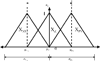

FIGURE 30.3 Linear membership functions.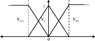

FIGURE 30.4 Linear-trapezoidal membership functions.

Otherwise, the membership value is equal to 1. Thus, we arrive at the membership functions shown in Fig. 30.4. Each region of the linear and trapezoidal-linear membership functions is distinguished from another by the different values of and L. One important criterion that should be taken into consideration is that the union of the domain of all membership functions for a given input must cover the entire range of the input [10]. Thus the trapezoidal modification is often employed to ensure coverage of the entire input space.

The Gaussian membership function is characterized by Eq. (30.2(b)). The Gaussian function can also be modified to form the trapezoidal-Gaussian function. In this case, if the input falls between the mean [Iq and zero, Eq. (30.2(b)) is used to find the membership value. Otherwise the membership value becomes 1. The Gaussian function is shown in Fig. 30.5 and the modified version is shown in Fig. 30.6.

A third type of membership function, known as the fuzzy singleton, is also considered. The fuzzy singleton is a special function in which the membership value is 1 for only one particular value of the linguistic input variable and zero otherwise [4]. Thus, the fuzzy singleton is a special case of the membership function with a width, cr, of zero. Therefore, the only parameter that needs to be defined is the mean, of the singleton. Thus, if the input is equal to [i, then the membership value is 1. Otherwise it is zero. We can denote the singleton membership function as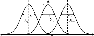

FIGURE 30.5 Gaussian membership functions.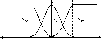

FIGURE 30.6 Gaussian-trapezoidal membership functions.

The fuzzy singleton function is quite useful in defining some special membership functions. If we would like to dispense with the need for a continuous degree of membership and prefer a binary valued function, the fuzzy singleton is an ideal candidate. We can form the membership function representing the fuzzy variable as a collection of fuzzy singletons ranging within the regions denoted by \\i + cr/2, - cr/2]. A graphical representation using three fuzzy variables (membership functions) is shown in Fig. 30.7 (In Fig. 30.7 the corners are only slanted so that the regions are easier to distinguish from each other.) Thus, the membership functions shown in Fig. 30.7 would be best defined as an integral of the fuzzy singleton with respect to the mean over the width of the function. Consequently, the membership function X(cr, [i) would be defined as follows:

X((7, [i) =

(30.6)

Jfi-a/2

where is the singleton function.