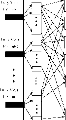Rul -1

Rul -3

Rul -5

Rul -k

-(wi,yi)

►(W2 , у2)

- (W3 , уз)

Fu у Out ut

-► (W4, У4)

- (W5, У5)

(Wk, ук)

FIGURE 30.8 Fuzzy inference engine.

30.2.3 The Fuzzy Inference Engine

The fuzzy inference engine uses the fuzzy vectors to evaluate the fuzzy rules and produce an output for each rule. Figure 30.8 shows a block diagram of the fuzzy inference engine. Note that the rule-based system takes the form found in Eq. (30.1). This form could be applied to traditional logic as well as fuzzy logic albeit with some modification. A typical rule R would be:

R: IF Xi THEN у = Q

(30.7)

where x is the result of some logic expression.

The logical expression used in the case of fuzzy inference (30.7) is of the form

xeXi

(30.8)

where x is the input and is the linguistic variable.

In binary logic, the expression in Eq. (30.8) results in either true or false. Fiowever, in fuzzy logic we often require a continuum of truth values. Figures 30.9 and 30.10 illustrate the difference between binary logic and fuzzy logic. In traditional logic, there is a single point representing the boundary between true and false. While in fuzzy logic, there is an entire

d t 1

Sftm t

Thr h Id P t

FIGURE 30.9 Binary logic statement evaluation.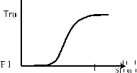

Thr hldRg

FIGURE 30.10 Fuzzy logic statement evaluation.

region over which there is a continuous variation between truth and falsehood. The second part of Eq. (30.7), у = Q, is the action prescribed by the particular rule. This portion indicates what value wiU be assigned to the output. This value could be either a fuzzy linguistic description or a crisp numerical value.

The logical expression that dictates whether the result of a particular rule is carried out could involve multiple criteria. Multiple conditions imply multiple input, as is most often the case in many applications of fuzzy logic to dynamic systems. Let us describe a system with two inputs x and x. For simphcity of explanation and without loss of generality, we wiU use 3 fuzzy variables, namely PV, ZE and NV. Although each linguistic variable x and x uses the same fuzzy quah-fiers, each input must have its own membership functions since they belong to different spaces. Thus, we wiU have two fuzzy vectors and x, for the first and second input, respectively:

x=[Xl,y(x) Xze(x)) xUx)] = [xl x\ xl]

(30.9(a))

= [Xly{x) xIe{x)) Xly{x)] = [x\ x\

(30.9(b))

where

Xy = membership function for the Negative fuzzy variable for input n = membership function for the Zero fuzzy variable for input n

Xpy = membership function for the Positive fuzzy variable for input n y} first linguistic variable (input 1) x second linguistic variable (input 2) x\ the degree of membership of input 1 into the ith fuzzy

variables category x} the degree of membership of input 2 into the jth fuzzy

variables category.

The inference mechanism in this case would be specified by the rule R.

IF (x\ AND x/) THEN у = Q.

(30.10)

The specification R is made so as to emphasize that all combinations of the components of the fuzzy vectors should be used in separate rules. A specific example of one of the rules can be described as follows:

Ri\ IF {x\ AND Хз) THEN / = C13.

This rule can be written linguistically as

Ri\ IF ((x is Negative AND is Positive))

THEN у =

where

y} is the first linguistic variable y? is the second hnguistic variable Ci3 is the output action to be defined by the system designer.

The AND in Eq. (30.10) can be interpreted and evaluated in two different ways. First, the AND could be evaluated as the product of X- and [7]. Thus

x\ AND x] = xjxf.

The second method is by taking the minimum of the terms [7]. In this case the result is the minimum value of the membership values. Therefore

xj AND xj = mm(xj, xj).

The most commonly used method in the literature is the product method. Therefore, the product method is used in this chapter to evaluate the AND function. Equation (30.10) can be expanded to multiple input with multiple fuzzy variables. In the most general case of n inputs and к linguistic qualifiers, we would have the rule Rf.

Rf IF [xj AND xj AND ... AND xf]

THEN y=Ci (30.11)

Recalhng that all combinations of input vector components must be taken between fuzzy vector components the system designer could have up to nk rules, where n is the number of fuzzy variables used to describe the inputs and к is the number of inputs. The number of rules used by the fuzzy inference engine could be reduced if the designer could eliminate some combinations of input conditions.

30.2.4 Defuzzification

The fuzzy inference engine as described previously often has multiple rules, each with possibly a different output. Deffuz-zification refers to the method employed to combine these

many outputs into a single output. Using Eq. (30.11) where multiple inputs (xx ... x ) should be evaluated, the product due to the evaluation of the premise conditions (defined by the components of the fuzzy vectors) determines the strength of the overall rule evaluation, wf.

Wi = xj AND xj AND .., w, = (xj)(xj)...(x)

(30.12)

where xf is the membership value of the kth input into the ith fuzzy variables category. This value, Wp becomes extremely important in defuzzification. Ultimately, defuzzification involves both the set of outputs Q and the corresponding rule strength w.

There are a number of methods used for defuzzification, including the center of gravity (COG) and mean of maxima (MOM) [13]. The COG method otherwise known as the fuzzy centroid is denoted by y.

cog T.iiQ

(30.13)

where w = Ylk Q is the corresponding output.

The mean of maxima method selects the outputs Q that have the corresponding highest values of w.

.MOM

= E Q/Car(G)

(30.14)

where G denotes a subset of Q consisting of these values that have the maximum value of w.

Out of the two methods of defuzzification, the most common method is the fuzzy centroid and is the one employed in this chapter.

30.3 Applications of Fuzzy Logic to Electric Drives

High performance drives require that the shaft speed and the rotor position follow pre-selected tracks (trajectories) at all times [11,12]. To accomplish this, two fuzzy control systems were designed and implemented. The goal of fuzzy control system is to replace an experienced human operator with a fuzzy rule-based system. The fuzzy logic controller provides an algorithm that converts the linguistic control maneuvering, based on expert knowledge, into an automatic control approach. In this section, a Fuzzy Logic Controller (FLC) is proposed and applied to high performance speed and position tracking of a brushless dc (BLDC) motor. The proposed controller provides the high degree of accuracy required by high performance drives without the need for detailed mathematical models. A laboratory implementation of the fuzzy logic-tracking controller using the Motorola MC68HC11E9

microprocessor is described in this chapter. AdditionaUy, in this experiment a bang-bang controUer is compared to the fuzzy controUer.

30.3.1 Fuzzy Logic-Based Microprocessor Controller

The first step in designing a fuzzy controUer is to decide which state variables representative of system dynamic performance can be taken as the input signals to the controUer. Further, choosing the proper fuzzy variables formulating the fuzzy control rules are also significant factors in the performance of the fuzzy control system. Empirical knowledge and engineering intuition play an important role in choosing fuzzy variables and their corresponding membership functions. The motor drives state variables and their corresponding errors are usually used as the fuzzy controUers inputs including rotor speed, rotor position and rotor acceleration. After choosing proper linguistic variables as input and output of the fuzzy controller, it is required to decide on the fuzzy variables to be used. These variables transform the numerical values of the input of the fuzzy controUer to fuzzy quantities. The number of these fuzzy variables specifies the quality of the control, which can be achieved using the fuzzy controUer. As the number of the fuzzy variable increases, the management of the rules is more involved and the tuning of the fuzzy controller is less straightforward. Accordingly, a compromise between the quality of control and computational time is required to choose the number of fuzzy variables. For the BLDC motor drive under study two inputs are usually required. After specifying the fuzzy sets, it is required to determine the membership functions for these sets. Finally, the EEC is implemented by using a set of fuzzy decision rules. After the rules are evaluated, a fuzzy centroid is used to determine the fuzzy control output. DetaUs of the design of the proposed controUers are given in the following subsections.

30.3.2 Fuzzy Logic-Based Speed Controller

In the case of shaft speed control to achieve optimal tracking performance, the motor speed error (co) and the motor acceleration error (a) are used as inputs to the proposed controller. The controller output is the change in the motor voltage. For the fuzzy logic based speed controUer, the two inputs required are defined as

(30.15) (30.16)

aj.gf = 0, because we want to minimize the acceleration to zero

(X = the calculated acceleration in (rad/s).

For both the speed and acceleration errors, three regions of operation are established according to the fuzzy variables. These regions are positive error, zero and negative error. The proposed controUer uses these regions to determine the required motor voltage, which enables the motor speed to foUow a desired reference trajectory. Examples of the broad fuzzy decisions are:

IF speed error is positive, TFLEN decrease the output IF speed error is zero, TFLEN maintain the output IF speed error is negative, TFLEN increase the output IF acceleration error is positive, TFLEN decrease the output

IF acceleration error is zero, TFLEN maintain the output IF acceleration error is negative, TFLEN increase the output.

To achieve a sufficiently good quality of control, the three basic variables must be further refined. Thus the linguistic variable acceleration error has seven fuzzy variables: negative large (NL), negative medium (NM), negative smaU (NS), zero, positive smaU (PS), positive medium (PM) and positive large (PL). The values associated with the fuzzy variables for the acceleration error are shown in Table 30.2.

The linguistic variable speed error has nine fuzzy variables: negative large (NL), negative medium (NM), negative medium smaU (NMS), negative smaU (NS), zero, positive smaU (PS), positive medium (PM), positive medium smaU (PMS) and positive large (PL). Two fuzzy sets, namely negative medium smaU (NMS) and positive medium smaU (PMS), are added to enhance the tracking performance. The regions defined for each fuzzy variable for the speed error is summarized in Table 30.3.

After specifying the fuzzy sets, it is required to determine the membership functions for these sets. The membership function for the fuzzy variable representing ZERO is a fuzzy singleton. Additionally, the other membership functions are of the type described in Eq. (30.6) and are composed of fuzzy singletons within the region defined for each particular fuzzy

TABLE 30.2 Fuzzy variables for the acceleration error (a) for speed control

where

cOj-gf = the desired speed (rad/s) co = the measured speed (rad/s)

TABLE 30.3 Fuzzy variables for the speed error (cOg) for speed control

TABLE 30.4 Decision table for speed control

Velocity Error

NL NM NMS NS ZERO PS PMS PM PL Acceleration Error

PL NS NWS PWS PVS PS PMS PM PL PWL

PM NMS NVS ZERO PWS PVS PS PMS PML PVL

PS NMS NS NWS ZERO PWS PVS PS PM PL

ZERO NML NMS NVS NWS NWS ZERO PWS PVS PMS PML

NS NL NM NS NVS ZERO PWS PS PML

NM NVL NML NMS NS NVS NWS ZERO PVS PMS

NL NWL NL NM NMS NS NVS NWS PWS PS

variable. Figures 30.11 and 30.12 show the resulting membership function for the acceleration and speed errors, respectively.

The two fuzzy sets illustrated in Figures 30.11 and 30.12 result in 63 linguistic rules for the BLDC drive system under study. The conditional rules listed in Table 30.4 are clearly implied, and the physical meanings of some rules are briefly explained as follows:

Rule 1: IF speed error is PL (positive large) AND acceleration is PS (positive small), THEN change in control voltage (output of fuzzy controller) is PL (positive large). This rule implies a general condition when the measured speed is far from the desired reference speed. Accordingly, it requires a large increase in the control voltage to force the shaft speed to the desired reference speed quickly.

1

-738 -369 0 369 738

Acc 1 r t rr r (r d/ с 2)

FIGURE 30.11 Membership functions for the acceleration error.

-209 -104 -49

49 104 204

S d rr r (r d/ c)

FIGURE 30.12 Membership functions for the speed error.

Rule 2: IF speed error is PS (positive small) AND acceleration is ZERO, THEN change in control voltage is PWS (positive very very small). This rule implements the conditions when the error starts to decrease and the measured speed is approaching the desired reference speed. Consequently, a very small increase in the control voltage is applied.

Rule 3: IF speed error is ZERO AND acceleration is NS (negative small), THEN change in control voltage is PWS (positive very very small). This rule deals with the circumstances when overshoot does occur. A very small decrease in the control voltage is required, which brings the motor speed to the desired reference speed.

These rules comprise the decision mechanism for the fuzzy speed controller. The decision table. Table 30.4, consists of values showing the different situations experienced by the drive system and the corresponding control input functions. It is clear that each entry in Table 30.4 represents a particular rule.

Now it is necessary to find the fuzzy output (change in control voltage). In this experiment the fuzzy centroid is used. Equation (30.17) shows the fuzzy centroid used to compute the final output of the controller:

output =

WjOi + W2O2 + W3O3

М/бзОбз

Wi + W2 + W3 H-----h W63

(30.17)

The weights will be the strength of each particular rules evaluation. The rule strength is evaluated as the product of the membership values associated with the speed and acceleration errors for the particular fuzzy variables involved in that rule. Since the membership functions were comprised solely of fuzzy singletons and the AND operator is evaluated as a product, the strength of each rules evaluation (w) will be either 0 or 1. Additionally, since the membership functions do not overlap, only one rule will be evaluated as true at each sample time. Thus all the weights will be zero except one. So the actual implementation can be simplified.

(30.18) (30.19)

= the measured speed in radians/s.

Nine fuzzy variables were defined for the position error and seven for the speed error. The fuzzy variables for the position error and the speed are defined in Tables 30.5 and 30.6, respectively. After specifying the fuzzy sets for the position controller, the membership functions can then be fully defined if it is required to determine the membership functions for these sets. The membership function for the fuzzy variable ZERO is a fuzzy singleton. Additionally, the other membership functions are of the type described in Eq. (30.6) and are composed of fuzzy singletons within the region defined for each particular fuzzy variable. Figures 30.13 and 30.14 show the resulting membership function for the speed and position errors respectively.

A corresponding output to the motor based on the speed and the rotor position error detected in each samphng interval must be assigned and thereby specifying the fuzzy inference engine. This is done by the fuzzy rules. For example, IF the position error is PL (positive large) AND the speed is PS (positive smaU), TFiEN a large positive change in driving effort is used. The crisp (defuzzified) output signal of the fuzzy controUer is obtained by calculating the centriod of aU fuzzy output variables. The fuzzy rule-base, on which the required change in the motor voltage is generated, is illustrated in Table 30.7.

TABLE 30.5 Fuzzy variables of the speed error for position control

TABLE 30.6 Fuzzy variables of position error {в^) for position control

= ref act

where

0 = the desired position in radians 0 = the measured position in radians

cOj-gf = 0, because we want to minimize the speed to zero \

-209

-104

104 209

S d rrr (rd/ c)

FIGURE 30.13 Membership functions for the speed error.

В

-2.21 -1.05 -0.53 0 0.53 1.05 2.21 P t rrr(rd)

FIGURE 30.14 Membership functions for the position error.

TABLE 30.7 Decision table for position control

Position Error

NMS NS ZERO PS

PMS PM PL

Speed Error

PL NS NWS

PM NMS NVS

PS NMS NS

ZERO NML NMS

NS NL NM

NM NVL NML

NL NWL NL

PWS PVS PS PMS PM PL PWL

ZERO PWS PVS PS PMS PML PVL

NWS ZERO PWS PVS PS PM PL

NVS NWS ZERO PWS PVS PMS PML

NS NVS NWS ZERO PWS PS PML

NMS NS NVS NWS ZERO PVS PMS

NM NMS NS NVS NWS PWS PS

30.3.3 Fuzzy Logic-Based Position Controller

The task of the position control algorithm is to force the rotor position of the motor to foUow a desired reference track without overshoot. The same method applied to the fuzzy speed controller is applied to the position controller. The inputs to the fuzzy position controller are, angular position error and motor speed error (ш^). The output from the controller is a change in the motor voltage. The two inputs are defined as foUows:

30.4 Hardware System Description

The BLDC drive system under control consists of the components illustrated in Figure 30.15. The drive system is made up of several distinct subsystems: the motor, a personal computer (PC), the driving circuit, and the microprocessor evaluation board. The motor is A HP, 3000 rev/min BLDC motor, and was manufactured by Pittman Company. The BLDC motor is equipped with a hall-effect sensor and an incremental optical encoder. The hall-effect sensors detect the rotor position to indicate which of the three phases of the motor is to be excited as the motor spins. The optical position encoder with resolution of 500 pulses/revolution is used to give speed and position feedback.

The controller is implemented by software and executed using a microprocessor. The control algorithm is written and loaded into the microprocessor using the PC. The computer used is an IBM 486 PC. The driving circuit is constructed using two major components: (1) the integrated circuit (UDN2936W-120) designed for BLDC drives [1], and (2) the digital to analog converter (DAC) and power amplifier. The inputs to the integrated circuit are the rotor position (which is obtained from Hall-effect sensors), the direction of desired rotation, and the magnitude of the control voltage. The output of the switching logic section is a sequence of gating signals that are pulse width-modulated (PWM). These signals are used to drive the power converter portion of the chip. The power converter is a dc/ac inverter utilizing 6 MOSFETs. The output of the power converter is a chopped three-phase ac waveform.

The microprocessor used was the Motorola MC68HC11E9 microprocessor [9]. The onboard memory system includes 8 kbytes of ROM (read-only memory), 512 bytes of EEPROM (electrically erasable programmable ROM), and 256 bytes of RAM (random access memory). The processor also has four 8

bit parallel input/output ports, namely A, B, С and E. The program is completely contained in the microprocessor and the computer is only required to load new programs into the processor. Additionally, it has an internal analog-to-digital converter, and can accept up to four analog inputs. Figure 30.15 includes the integrated circuit (UDN2936W-120) designed for operating the BLDC motor. The range of the input voltage (control voltage) is between zero and 25 V. The motor speed for any control voltage less than 7 V is zero. This indicates that the motor requires a minimum of 7 V to start. This limitation is actually a protective feature of the circuit to prevent malfunctions [1]. Thus, the actual output of the microprocessor (the control signal Vc(/c)) is added to a 7V dc offset, using a summing amphfier. The current out of the summing amphfier must first be increased before it can be used to drive the motor. The current amplification is accomplished by using a 40 V power transistor (TIP31A). In addition, when a sudden change in speed or direction occurs, the back emf produced by the motor can sometimes cause large currents. Since the output stage of the integrated circuit (UDN2936W-120) has transistors with a current rating of ±3 A, some limiting resistors were needed to prevent damage. Figure 30.16 shows a snapshot of the laboratory experiment.

Speed measurements were taken using a frequency to voltage converter LM2907. The LM2907 produces a voltage proportional to the frequency of the pulses it receives at its input. In this experiment, the pulses were sourced from the encoder signal A. The circuit was constructed such that the maximum speed of the motor corresponded to 5 V. This value was input into the microprocessor, via the onchip A/D converter, as an 8 bit word. The direction of rotation was observed using a D flipflop. This direction signal was used to indicate the sign of the speed. The two signals, speed and direction, were combined within the software environment to

R r с

Trek

M cr r с r vlut В rd

trlSgl / V (k) /

tgrtd rcut

/ (U N2936-120)

Swtch g Lgc

F dbck

P t cdr

S d V rt r

fBm hi Mtr

produce an integer. Thus internaUy the speed could range from +256 to -256. These limits represent +3000 and -3000 r.p.m., respectively. Additionally, the digital output of the microprocessor was limited to the resolution provided by 7 bits. Therefore, if the desired output voltage was 22 V, then the maximum byte output was 127. Thus each increment in control signal, numerically within the microprocessor, would produce a change of 0.17 V.

30.4.1 Experimental Results

A square wave foUowed by a sinusoidal reference track was considered. In this experiment, there is a weight attached to the motor via a cable and puUey assembly. Figure 30.17 shows the speed tracking performance of the fuzzy logic controller. The motor is under constant load. The actual motor speed is superimposed on the desired reference speed in order to compare tracking accuracy. High tracking accuracy is observed at aU speeds. The corresponding position tracking performance is displayed in Figure 30.18. Reasonable position tracking accuracy is displayed. One can see from these figures that the results were very successful. For comparison purposes. Figs. 30.19 and 30.20 exhibit cases in which the fuzzy logic controUer was replaced by a bang-bang controUer. However,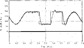

FIGURE 30.17 Fuzzy speed tracking under loading condition.

6.45 5.16 3.87 2.58 Й 1.29 0.00

0 0.5 1.0 1.5 2.0 2.5 3.0 3.5 4.0 4.5 5.0 Tm (Sc)

FIGURE 30.18 Fuzzy position tracking under loading condition.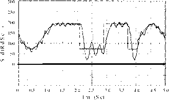

FIGURE 30.19 Bang-bang speed tracking under loading condition.

5.16

3.87

2.58

1.29 0.00

0 0.5 1.0 1.5 2.0 2.5 3.0 3.5 4.0 4.5 5. Tm (Sc)

FIGURE 30.20 Bang-bang position tracking with load.

when a bang-bang controUer was applied the controller could not maintain tracking accuracy. That is, the response using the bang-bang controller was unsatisfactory.

30.5 Conclusion

This chapter describes a fuzzy logic-based microprocessor controUer, which incorporates attractive features such as simphcity, good performance, and automation whUe utUizing a low cost hardware and software implementation. The test results indicate that the fuzzy logic-tracking controUers foUow the trajectories successfully. Additionally, experimental results show that the effective smooth speed/position control and tracking of BLDC motors can be achieved by the EEC, thus making it suitable for high performance motor drive applications. The controller design does not require exphcit knowledge of the motor/load dynamics. This is a useful feature when dealing with parameter and load uncertainties. The advantage of using a fuzzy logic-tracking controUer in this application is that it is weU suited to the control of unknown or iU-defined nonlinear dynamics.

Acknowledgments

The author would like to acknowledge the assistance of Mr Daniel О Ricketts, a graduate student at Howard University, in clarifying these concepts and obtaining the experimental results. The author would also like to acknowledge the financial support by NASA Glenn Research Center, in the form of grant no. NAG3-2287 technically monitored by Mr Donald F Noga.

References

1. Allegro. (1993) UDN2936W-120 Technical Data Manual

2. Mitra, S and Pal. K. S. (1996). Fuzzy self-organization, inferencing, and rule generation, IEEE Trans. Syst, Man, and Cybern.-Part A: Syst Humans 26(5), 608-619.

3. Jamshidi, M., Vadiee, N. and Ross, T. (1993) Fuzzy Logic and Control, Prentice Hall, Englewood Cliffs, NJ.

4. Lee, C. C. (1990). Fuzzy logic in control systems: fuzzy logic controller. Part I. IEEE Trans. Syst Man, and Cybernetics 20(2), 404-418.

5. Lee, J. (1993). On methods for improving performance of Pl-type fuzzy logic controllers. IEEE Trans. Fuzzy Systems 1(4), 298-301.

6. Lofti, A., and Tsoi, A. C. (1996). Learning fuzzy inference systems using an adaptive membership function scheme. IEEE Trans. Syst, Man and Cybernetics 26(2), 326-331.

7. Lofti, A., Andersen H. C. and Tsoi, A. C. (1996). Matrix formulation of fuzzy rule-based systems. IEEE Trans. Syst, Man and Cybernetics 26(2), 332-339.

8. Marks II, R. J. (ed.) (1994). Fuzzy Logic Technology and Applications IEEE Press, New York.

9. Motorola. (1995) MC68HC11E9 Technical Data Manual.

10. Ross, T. J. (1995). Fuzzy Logic with Engineering Applications McGraw-Hill, New York.

11. Rubaai, A. and Kotaru, R. (1999). Neural net-based robust controller design for brushless DC motor drives. IEEE Trans. Syst, Man and Cybernetics, Part C: Applications and Review 29(3), pp. 460-474.

12. Rubaai, A. Kotaru, R. and Kankam, M. D. (2000). A continually online-trained neural network controller for brushless DC motor drives. IEEE Trans. Ind. Appl. 36(2), 475-483.

13. Ross, T. J. (1995). Fuzzy Logic with Engineering Applications McGraw-Hill, New York.

14. Zadeh, L. (1973). Outline of a new approach to the analysis of complex systems and decision processes. IEEE Trans. Syst Man and Cybernetics, 3(1), 28-44.

Automotive Applications of Power Electronics

David J. Perreault, Ph.D.

Massachusetts Institute of Technology, Laboratory for Electromagnetic and Electronic Systems 77 Massachusetts Avenue, 10-039 Cambridge, Massachusetts 02139, USA

Khurram K. Afridi, Ph.D.

Techlogix, 800 West Cummings Park, 1200, Woburn, Massachusetts 01801, USA

Iftikhar A. Khan, Ph.D.

Delphi Automotive Systems 2705 South Goyer Road, MS D35, Kokomo, Indiana USA

31.1 Introduction..................................................................................... 791

31.2 The Present Automotive Electrical Power System................................... 792

31.3 System Environment.......................................................................... 792

31.3.1 Static Voltage Ranges 31.3.2 Transients and Electromagnetic Immunity

31.3.3 Electromagnetic Interference 31.3.4 Environmental Considerations

31.4 Functions Enabled by Power Electronics............................................... 797

31.4.1 High Intensity Discharge Lamps 31.4.2 Pulse-Width Modulated Incandescent Lighting 31.4.3 Piezoelectric Ultrasonic Actuators 31.4.4 Electromechanical Engine Valves 31.4.5 Electric Air Conditioner 31.4.6 Electric and Electro-Hydraulic Power Steering Systems 31.4.7 Motor Speed Control

31.5 Multiplexed Load Control.................................................................. 801

31.6 Electromechanical Power Conversion................................................... 803

31.6.1 The Lundell Alternator 31.6.2 Advanced Lundell Alternator Design Techniques

31.6.3 Alternative Machines and Power Electronics

31.7 Dual/FLigh Voltage Automotive Electrical Systems.................................. 808

31.7.1 Trends Driving System Evolution 31.7.2 Voltage Specifications

31.7.3 Dual-Voltage Architectures

31.8 Electric and Hybrid Electric Vehicles.................................................... 812

31.9 Summary......................................................................................... 813

References........................................................................................ 814

31.1 Introduction

The modern automobile has an extensive electrical system consisting of a large number of electrical, electromechanical, and electronic loads that are central to vehicle operation, passenger safety, and comfort. Power electronics is playing an increasingly important role in automotive electrical systems - conditioning the power generated by the alternator, processing it appropriately for the vehicle electrical loads, and controlhng the operation of these loads. Furthermore, power electronics is an enabling technology for a wide range of future loads with new features and functions. Such loads include electromagnetic engine valves, active suspension, controlled lighting, and electric propulsion.

This chapter discusses the application and design of power electronics in automobiles. Section 31.2 provides an overview

of the architecture of the present automotive electrical power system. The next section, Section 31.3, describes the environmental factors, such as voltage ranges, EMI/EMC requirements, and temperature, which strongly influence the design of automotive power electronics. Section 31.4 discusses a number of electrical functions that are enabled by power electronics, while Section 31.5 addresses load control via multiplexed remote switching architectures that can be implemented with power electronic switching. Section 31.6 considers the application of power electronics in automotive electromechanical energy conversion, including power generation. Section 31.7 describes the potential evolution of automotive electrical systems towards high- and dual-voltage systems, and provides an overview of the likely requirements of power electronics in such systems. Finally, the apphcation of power electronics in electric and hybrid electric vehicles is addressed in Section 31.8.

31.2 The Present Automotive Electrical Power System

Present day automobiles can have over 200 individual electrical loads, with average power requirements in excess of 800 W. These include such functions as the headlamps, tail lamps, cabin lamps, starter, fuel pump, wiper, blower fan, fuel injector, transmission shift solenoids, horn, cigar lighter, seat heaters, engine control unit, cruise control, radio, and spark ignition. To power these loads present day internal combustion engine (ICE) automobiles use an electrical power system similar to the one shown in Fig. 31.1. Power is generated by an engine-driven three-phase wound-field synchronous machine - a Lundell (claw-pole) alternator [1, 2]. The ac voltage of this machine is rectified and the dc output regulated to about 14 V by an electronic regulator that controls the field current of the machine. The alternator provides power to the loads and charges a 12 V lead-acid battery. The battery provides the high power needed by such loads as the starter, and supphes power when the engine is not running or when the demand for electrical power exceeds the output power of the alternator. The battery also acts as a large capacitor and smoothes out the system voltage.

Power is distributed to the loads via fuses and point-to-point wiring. The fuses, located in one or more fuseboxes, protect the wires against overheating and fire in the case of a short. Most of the loads are controlled directly by manually actuated mechanical switches. These primary switches are located in areas in easy reach of either the driver or the passengers, such as the dashboard, door panels, and the ceihng. Some of the heavy loads, such as the starter, are switched indirectly via electromechanical relays.

31.3 System Environment

The challenging electrical and environmental conditions found in the modem automobile have a strong impact on the design of automotive power electronic equipment. Important factors affecting the design of electronics for this applica-

tion include static and transient voltage ranges, electromagnetic interference and compatibility requirements (EMI/EMC), mechanical vibration and shock, and temperature and other environmental conditions. This section briefly describes some of the factors that most strongly affect the design of power electronics for automotive apphcations. For more detailed guidehnes on the design of electronics for automotive applications, the reader is referred to [1, 3-16] and the documents cited therein, from which much of the information presented here is drawn.

31.3.1 Static Voltage Ranges

In most present-day automobiles, a Lundell-type alternator provides dc electrical power with a lead-acid battery for energy storage and buffering. The nominal battery voltage is 12.6 V, which the alternator regulates to 14.2 V when the engine is on in order to maintain a high state of charge on the battery. In practice, the regulation voltage is adjusted for temperature to match the battery characteristics. For example, in [1], a 25°C regulation voltage of 14.5 V is specified with a - 10 mV/°C adjustment. Under normal operating conditions, the bus voltage will be maintained in the range of 11-16 V [3]. Safety-critical equipment is typically expected to be operable even under battery discharge down to 9V, and equipment operating during starting may see a bus vohage as low as 4.5-6 V under certain conditions.

In addition to the normal operating voltage range, a wider range of conditions is sometimes considered in the design of automotive electronics [3]. One possible condition is reverse-polarity battery installation, resulting in a bus voltage of approximately -12 V. Another static overvoltage condition can occur during jump starting from a 24 V system such as on a tow truck. Other static overvoltage conditions can occur due to failure of the alternator voltage regulator. This can result in a bus voltage as high as 18 V, followed by battery electrolyte boil-off and a subsequent unregulated bus voltage as high as 130 V. Typically, it is not practical to design the electronics for operation under such an extreme fault condition, but it should be noted that such conditions can occur. Table 31.1

Alternator

Battery

Primary Fusebox Switches

Loads

\ Relay

FIGURE 31.1 The 12 V point-to-point automotive electrical power system.