FIGURE 32.10 Capacitor switching transient.

32.2.7 Monitoring and Measurement

To consider or be able to diagnose power quality related problems, it is imperative to be able to measure various power quality parameters. Several different categories of monitoring and measurement equipment exist for these purposes, with costs ranging from a few hundred doUars to $10,000-$20,000 for fully equipped disturbance analyzers.

The most basic category of power quality measurement tool is the hand-held voltmeter. It is important that the voltmeter be a true-rms meter, or erroneous readings wiU be obtained that incorrectly suggest low or high voltage when harmonics are present in the signal. It is especially important to have true rms capability when measuring currents; voltage distortion is not typically severe enough to create large errors in the readings of non-true-rms meters. Virtually aU major measurement equipment vendors offer true-rms meters, with costs starting around $100.

The next step up from the basic voltmeter is a class of instruments that have come to be caUed power quality analyzers. These instruments are hand held and battery powered. These instruments can measure and display various power quality indices, especially those that relate to harmonics like TFiD, etc., and can also display the input waveform. Newer models feature 20 MFiz (and higher) bandwidth osciUoscopes, inrush measurements, time trending, and other useful features. Manufacturers such as Fluke, Dranetz, BMI, and Tektronix offer these types of instruments for around $2,000.

In most power quality investigations, it is not possible to use hand-held equipment to coUect sufficient data to solve the problem. Most power quality problems are intermittent in nature, so some type of long-term monitoring is usually required. Various recorders are available that can measure and record voltage, current, and power over user-defined time periods. Such recorders typically cost on the order of $3,000-$ 10,000. More advanced long-term monitors can

record numerous power quality events and indices, including transients, harmonics, sags, flicker, etc. These devices, often caUed line disturbance analyzers typically cost between $10,000-$20,000.

It is important to use the right instrument to measure the phenomenon that is suspected of causing the problem. Some meters record specific parameters, while others are more flexible. With this flexibility comes an increased learning curve for the user, so it is important to spend time on them before going out to monitor to make sure aU aspects and features of the equipment are understood.

It is equally important to measure in the correct location. The best place to measure power quality events is at the equipment terminals that are experiencing problems. With experience, an engineer can evaluate the waveforms recorded at the equipment terminals and correlate them to events and causes elsewhere in the power system. In general, the farther away from the equipment location the monitoring takes place, the more difficult it can be to diagnose a problem.

32.3 Reactive Power and Harmonic Compensation

The previous section specifically identified harmonics as a potential power quality problem. In that discussion, it was pointed out that nonlinear loads such as adjustable speed drives create harmonic currents, and when these currents flow through the impedances of the power supply system, harmonic voltages are produced. While harmonic currents have secondary (in most cases) negative impacts, it is these harmonic voltages that can be supplied to other load equipment (and disrupt operation) that are of primary concern. Fiaving parallel or series resonant conditions present in the electrical supply system can quickly exacerbate the problem.

32.3.1 Typical Harmonics Produced by Equipment

In theory, most harmonic currents foUow the 1 / n rule where n is the harmonic order (180 Fiz = 3 x 60; n = 3). Also in theory, most harmonic currents in three-phase systems are not integer multiples of three. Finally, in theory, harmonic currents are not usually even-order integer multiples of the fundamental. In practice, none of these statements are completely true and using any of them exactly could lead to either over- or under-conservatism depending on many factors. Consider the foUowing examples:

1. Switched-mode power supplies, such as found in televisions, personal computers, etc., often produce a third harmonic current that is nearly as large (80-90%) as the fundamental frequency component.

2. Unbalance in voltages supphed to a three-phase converter load wiU lead to the production of even-

order harmonics and, in some extreme cases, estabhsh a positive feedback situation leading to stability problems.

3. Arcing loads, particularly in the steel industry, generate significant harmonics of all orders, including harmonics that are not integer multiples of the power frequency.

4. Cycloconverters produce dominant harmonics that are integer multiples of the power frequency, but they also produce sideband components at frequencies that are not integer multiples of the power frequency. In some control schemes, the amplitudes of the sideband components can reach damaging levels.

Table 32.2 gives the magnitudes, in percent of fundamental, of the first 25 (integer) harmonics for a single-phase switched-mode power supply, a single-phase fluorescent lamp, a three-phase (six-pulse) dc drive, and a three-phase (six pulse, no input choke) ac drive. Together, these load types represent the range of harmonic sources in power systems. Note that seemingly minor changes in parameter values and control methods can have significant impacts on harmonic current generation; the values given here are on the conservative side of typical.

32.3.2 Resonance

Considering only the harmonic current spectra given in Table 32.2, it would appear that a large number of harmonic-related

power quality problems are on the verge of appearing. In reality, most current drawn by many residential, commercial, and industrial customers is of the fundamental frequency; the amplitudes of the individual harmonic currents, in percent of the total fundamental current, are often much less than what is shown in Table 32.2. For this reason, end-use locations employing nonhnear loads often do not lead directly to significant voltage distortion problems. A parallel resonance in the power supply system, however, changes the picture entirely.

Series and parallel resonance exist in any ac power supply network that contains inductance(s) and capacitance(s). The following simple (but useable) definitions apply:

1. Series resonance occurs when the impedance to current flow at a certain frequency (or frequencies) is low.

2. Parallel resonance occurs when the impedance to current flow at a certain frequency (or frequencies) is high.

For a given harmonic-producing load that generates harmonics at frequencies that correspond to parallel resonance in the supply system, even small currents at the resonant frequencies can produce excessive voltages at these same frequencies. The principle of series resonance, however, is usually exploited to reduce harmonics in power systems by providing intentionally low impedance paths to ground.

In many cases, end-users will install power factor correction capacitors in order to minimize reactive power charges by the

TABLE 32.2 Typical harmonic spectra of load equipment

supply utility. In most cases, these capacitors are located on the customers low voltage supply buses and are therefore in paraUel with the service transformer. In most cases where the power factor correction capacitors are sized to provide a net power factor (at the service entrance) to 0.85 (lag) -1.0, the paraUel resonance occurs somewhere between the 5th and 9th harmonic. Considering Table 32.2, it is apparent that a large number of loads produce harmonics at these frequencies, and the amplitudes can be significant. Even a smaU increase in impedance at these frequencies due to resonance can lead to unacceptable voltages being produced at these same frequencies. Figure 32.11 shows an example plot of impedance looking into a UtUity supply system when a typically-sized capacitor bank has been instaUed to improve overaU plant power factor.

From Figure 32.11, it is clear that l.OA at the 9th harmonic wiU produce at least 150 times more voltage drop than would be produced by the same 1.0 A if it were at the fundamental frequency. A look back at Table 32.2 shows the clear potential for problems. Fortunately, the series resonance principle can be used to provide a low impedance path to ground for the harmonic currents and thus reduce the potential for problematic voltage distortion.

Because capacitors are required to produce paraUel resonance, it is often a cheap fix to slightly modify the capacitor to include a properly sized series reactor and create a filter. This filter approach, designed based on the series resonance concept, is usually the most cost-effective means to control harmonic voltage distortion.

32.3.3 Harmonic Filters

Fiarmonic filters come in many shapes and sizes. In general, harmonic filters are shunt filters because they are connected in paraUel with the power system and provide low impedance paths to ground for currents at one or more harmonic frequencies. For power apphcations, shunt filters are almost always more economical than series filters (like those found in many communications apphcations) for the foUowing reasons:

1. Series components must be rated for the fuU current, including the power frequency component. Such a requirement leads to larger component sizes and therefore costs.

2. Shunt filter components generally must be rated for only part of the system voltage (usually with respect to ground). Such requirements lead to smaUer component sizes and therefore costs.

Shunt filters are designed (or can be purchased) in three basic categories as follows:

1. single-tuned filters,

2. multiple- (usually hmited to double) tuned filters, and

3. damped filters (of first, second, or third order, or newer c type ).

The single- and double-tuned filters are usually used to filter specific frequencies, whUe the damped filters are used to filter a wide range of frequencies. In applications involving smaU harmonic producing loads, it is often possible to use one single-tuned filter (usually tuned near the 5th harmonic) to eliminate problematic harmonic currents. In large applications, like those associated with arc furnaces, multiple tuned filters and a damped filter are often used. Equivalent circuits for single- and double-tuned filters are shown in Figure 32.12. Equivalent circuits for first, second, third, and c type damped filters are shown in Figure 32.13.

A plot of the impedance as a function of frequency for a single-tuned filter is shown in Figure 32.14. The filter is based on a 480 V, 300 kvar (three-phase) capacitor bank and is tuned to the 4.7th harmonic with a quality factor, Q, of 150. Note that the quality factor is a measure of the sharpness of the tuning and is defined as X/R where X is the inductive reactance for the filter inductor at the (undamped) resonant frequency; typically 50 < Q < 150 for tuned filters.

A plot of impedance as a function of frequency for a second-order damped filter is shown in Figure 32.15. This filter is based on a 480 V, 300 kvar capacitor bank and is tuned to the 12th harmonic. The quality factor is chosen to be 1.5. Note that the quality factor for damped filters is the inverse of the definition for tuned filters; Q = R/X where X is the

cd О С CO D cd Q. £

Driving Point Impedance

Frequency (Hz) FIGURE 32.11 Driving point impedance.

(a) (b)

FIGURE 32.12 Single-tuned (a) and double-tuned (b) harmonic fihers.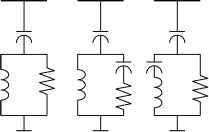

(a) (b) (c) (d)

FIGURE 32.13 Damped filters: first (a), second (b), and third (c) order, and с type (d).

inductive reactance at the (undamped) resonant fi-equency. Typically, 0.5 < Q < 1.5 for damped filters.

In most cases, it is common to tune single-tuned filter banks to shghtly below (typically around 5%) the frequency of the harmonic to be removed. The reasons for this practice are as follows:

1. For a low-resistance series resonance filter that is exactly tuned to a harmonic frequency, the filter bank will act as a sink to all harmonics (at the tuned frequency) in the power system, regardless of their source(s). This action can quickly overload the filter.

2. All electrical components have some nonzero temperature coefficient, and capacitors are the most temperature sensitive component in a tuned filter. Because most capacitors have a negative temperature coefficient (capacitance decreases and tuned frequency therefore increases with temperature), tuning shghtly lower than the desired frequency is desirable.

Damped filters are typically used to control higher-order harmonics as a group. In general, damped filters are tuned in between corresponding pairs of harmonics (11th and 13th, 17th and 19th, etc.) to provide the maximum harmonic reduction at those frequencies while continuing to serve as a (not quite as effective) filter bank for frequencies higher than the tuned frequency. Because damped filters have significantly higher resistance than single- or double-tuned filters, they are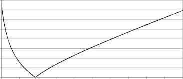

Frequency (Hz) FIGURE 32.14 Single-tuned fiher frequency response.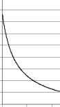

Frequency (Hz)

FIGURE 32.15 Second-order damped filter frequency response.

usually not used to filter harmonics near the power fi-equency so that filter losses can be maintained at low values.

32.4 IEEE Standards

The IEEE has produced numerous standards relating to the various power quality phenomena discussed in Section 32.2. Of these many standards, the one most appropriate to power electronic equipment is IEEE Standard 519-1992. This standard is actually a recommended practice, which means that the information contained within represents a set of recommendations, rather than a set of requirements. In practice, this seemingly smaU difference in wording means that the harmonic limits prescribed are merely suggested values; they are not (nor were they ever intended to be) absolute limits that could not be exceeded.

Harmonic control via IEEE 519-1992 is based on the concept that aU parties use and pay for the public power supply network. Due to the nature of utility company rate structures, end-users that have a higher demand pay more of the total infrastructure cost through higher demand charges. In this light, IEEE 519-1992 allows these larger end-users to produce a greater percentage of the maximum level of harmonics that can be absorbed by the supply utility before voltage distortion problems are encountered. Because the ability for a harmonic source to produce voltage distortion is directly dependent on the supply system impedance up to the point where distortion is to be evaluated, it is necessary to consider both

1. the size of the end-user and

2. the strength (impedance) of the system

at the same time in order to establish meaningful limits for harmonic emissions. Furthermore, it is necessary to establish tighter limits in higher voltage supply systems than lower voltage because the potential for more widespread problems associated with high voltage portions of the supply system.

Unlike limits set forth in various lEC Standards, IEEE 519-1992 established the point of common coupling, or PCC, as the point at which harmonic limits shaU be evaluated. In most cases (recaU that IEEE 519-1992 is a recommended practice ), this point wiU be:

1. in the supply system owned by the utility company,

2. the closest electrical point to the end-users premises, and

3. as in (2), but further restricted to points where other customers are (or could be in the future) provided with electric service.

In this context, IEEE 519-1992 harmonic limits are designed for an entire facility and should not be apphed to individual pieces of equipment without great care.

Because the PCC is used to evaluate harmonic limit compliance, the system strength (impedance) is measured at this point and is described in terms of available (three-phase) short-circuit current. Also, the end-users maximum average demand current is evaluated at this point. Maximum demand is evaluated based on one of the foUowing:

1. the maximum value of the 15 or 30 minute average demand, usually considering the previous 12 months bilhng history, or

2. the connected kVA or horsepower, perhaps multiplied by a diversity factor.

The ratio of Iq to 4 where Iq is the available fault current and 4 is the maximum demand current, implements the founding concept of IEEE 519-1992: larger end-users can create more harmonic currents, but the specific level of current that any end-user may produce is dependent on the strength of the system at the PCC. Tables 32.3-32.5 show the harmonic current limits in IEEE 519-1992 for various voltage levels.

In general, it is the responsibUity of the end-user to insure that their net harmonic currents at the PCC do not exceed the values given in the appropriate table. In some cases, usually associated with paraUel resonance involving a utility-owned capacitor bank, it is possible that aU customers wiU be within

TABLE 32.3 Current distortion limits for general distribution systems, 120V-69kV

Maximum Harmonic Current Distortion in Percent of Л

Individual Harmonic Order h (Odd Harmonics)

Even harmonics are limited to 25% of the odd harmonic limits above. Current distortions that result in a dc offset are not allowed.

AU power generation equipment is limited to these values of current distortion regardless of the value of Ic/h-

TABLE 32.4 Current distortion limits for general subtransmission systems, 69.001-161 kV

Maximum Harmonic Current Distortion in Percent of 4 Individual Harmonic Order h (Odd Harmonics)

32.5 Conclusions

Even harmonics are limited to 25% of the odd harmonic limits above. Current distortions that result in a dc offset are not allowed. AU power generation equipment is limited to these values of current distortion regardless of the value of /sc/4-

TABLE 32.5 Current distortion limits for general transmission systems, > 161 kV

Maximum Harmonic Current Distortion in Percent of 4 Individual Harmonic Order h (odd harmonics)

/sc l <11 n<h<\l \l<h<23 23</г<35 /г > 35 TDD

<50 2.0 1.0 >50 3.0 1.5

0.75 1.15

0.3 0.45

0.15 0.22

2.5 3.75

Even harmonics are limited to 25% of the odd harmonic limits above Current distortions that result in a dc offset are not allowed AU power generation equipment is limited to these values of current distortion regardless of the value of /sc/4-

TABLE 32.6 Vohage distortion hmits

the prescribed limits, but voltage distortion problems exist. In these cases, it is generally the responsibility of the supply utility to insure that excessive voltage distortion levels are not present. The harmonic voltage limits that are recommended for utility companies are given in Table 32.6.

In this chapter, various power quality phenomena have been described, with particular focus on the implications on power electronic converters and equipment. While one popular opinion blames power electronic equipment for causing most power quality problems, it is quite clear that power electronic converter systems can play an equally important role in reducing the impact of power quality problems. While it is true that power electronic converters and systems are the major cause of harmonic-related problems, the application (in general terms) of IEEE 519-1992 limits for current and voltage harmonics has led to the reduction, elimination, and prevention of most harmonic problems. Other power quality phenomena, like grounding, sags, and voltage flicker, are most often completely unrelated to power electronic systems. In reality, advances in power electronic circuits and control algorithms are making it more possible to control these events and minimize the financial impacts of the majority of power quality problems.

References

1. ANSI Std C84.1-1995, Electric Power Systems and Equipment-Voltage Ratings (60 Hz).

2. IEEE Std 493-1997, IEEE Recommended Practice for the Design of Reliable Industrial and Commercial Power Systems (IEEE Gold Book).

3. IEEE Std 142-1991, IEEE Recommended Practice for Grounding of Industrial and Commercial Power Systems (IEEE Green Book).

4. National Fire Protection Association 70-1999, National Electrical Code, 1999.

5. IEEE Std 519-1992, IEEE Recommended Practices and Requirements for Harmonic Control in Electrical Power Systems.

6. IEEE Std 141-1993, IEEE Recommended Practice for Electric Power Distribution for Industrial Plants (IEEE Red Book).

7. UIE Working Group WG2, J.L. Gutierrez Iglesias Chairman, Part 5: Fhcker and Vohage Fluctuations, 1999.

8. International Electrotechnical Commission, lEC Technical Report 61000-4-15, Flickermeter - Functional and Design Specifications, 1997.

9. IEEE Std 1100-1999, IEEE Recommended Practice for Powering and Grounding Electronic Equipment (IEEE Emerald Book).

10. IEEE Std 1159-1995, IEEE Recommended Practice for Monitoring Electric Power Quality.

11. Kimbark, Edward Wilson. Direct Current Transmission, vol. I. John Wiley & Sons, New York, 1948.

Active Filters

Luis Moran, Ph.D. Juan Dixon, Ph.D.

Dept. of Electrical Engineering Universidad de Concepcion Concepcion, Chile

33.1 Introduction...................................................................................... 829

33.2 Types of Active Power Filters................................................................ 829

33.3 Shunt Active Power Filters................................................................... 830

33.3.1 Power Circuit Topologies 33.3.2 Control Scheme 33.3.3 Power Circuit Design

33.4 Series Active Power Filters.................................................................... 841

33.4.1 Power Circuit Structure 33.4.2 Principles of Operation 33.4.3 Power Circuit

Design 33.4.4 Control Issues 33.4.5 Control Circuit Implementation 33.4.6 Experimental Results

References......................................................................................... 851

33.1 Introduction

The growing number of power electronics base equipment has produced an important impact on the quality of electric power supply. Both high power industrial loads and domestic loads cause harmonics in the network voltages. At the same time, much of the equipment causing the disturbances is quite sensitive to deviations from the ideal sinusoidal hne voltage. Therefore, power quality problems may originate in the system or may be caused by the consumer itself. Moreover, in the last years the growing concern related to power quality comes from:

Consumers that are becoming increasingly aware of the power quality issues and being more informed about the consequences of harmonics, interruptions, sags, switching transients, etc. Motivated by deregulation, they are chaUenging the energy suppliers to improve the quality of the power delivered.

The prohferation of load equipment with microprocessor-based controllers and power electronic devices which are sensitive to many types of power quality disturbances.

Emphasis on increasing overaU process productivity, which has led to the instaUation of high-efficiency equipment, such as adjustable speed drives and power factor correction equipment. This in turn has resulted in an increase in harmonics injected into the power system, causing concern about their impact on the system behavior.

For an increasing number of applications, conventional equipment is proving insufficient for mitigation of power quality problems. Fiarmonic distortion has traditionally been dealt with by the use of passive LC filters. Fiowever, the application of passive filters for harmonic reduction may result in paraUel resonances with the network impedance, over compensation of reactive power at fundamental frequency, and poor flexibUity for dynamic compensation of different frequency harmonic components.

The increased severity of power quality in power networks has attracted the attention of power engineers to develop dynamic and adjustable solutions to the power quality problems. Such equipment, generally known as active filters, are also caUed active power line conditioners, and are able to compensate current and voltage harmonics, reactive power, regulate terminal voltage, suppress flicker, and to improve voltage balance in three phase systems. The advantage of active filtering is that it automatically adapts to changes in the network and load fluctuations. They can compensate for several harmonic orders, and are not affected by major changes in network characteristics, eliminating the risk of resonance between the filter and network impedance. Another plus is that they take up very little space compared with traditional passive compensators.

33.2 Types of Active Power Filters

The technology of active power filter has been developed during the past two decades reaching maturity for harmonics

compensation, reactive power, and voltage balance in ac power networks. All active power filters are developed with PWM converters (current source or voltage source inverters). The current-fed PWM inverter bridge structure behaves as a nonsinusoidal current source to meet the harmonic current requirement of the nonlinear load. It has a self-supported dc reactor that ensures the continuous circulation of the dc current. They present good reliability, but have important losses and require higher values of parallel capacitor filters at the ac terminals to remove unwanted current harmonics. Moreover, they cannot be used in multilevel or multistep modes configurations to allow compensation in higher power ratings.

The other converter used in active power filter topologies is the voltage-source PWM inverter. This converter is more convenient for active power filtering applications since it is lighter, cheaper, and expandable to multilevel and multistep versions, to improve its performance for high power rating compensation with lower switching frequencies. The PWM voltage source inverter has to be connected to the ac mains through couphng reactors. An electrolytic capacitor keeps a dc voltage constant and ripple free.

Active power filters can be classified based on the type of converter, topology, control scheme, and compensation characteristics. The most popular classification is based on the topology such as shunt, series or hybrid. The hybrid configuration is a combination of passive and active compensation. The different active power filter topologies are shown in Fig. 33.1.

TABLE 33.1 Active filter solutions to power quality problems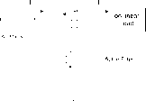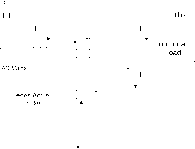

unt assi e Filter

FIGURE 33.1 Active power filter topologies implemented with PWM-VSI. (a) Shunt active power filter, (b) Series active power filter, (c) Hybrid active power filter.

Shunt active power filters (Fig. 33.1(a)) are widely used to compensate current harmonics, reactive power and load current unbalanced. It can also be used as a static var generator in power system networks for stabilizing and improving voltage profile. Series active power filters (Fig. 33.1(b)) is connected before the load in series with the ac mains, through a coupling transformer to eliminate voltage harmonics and to balance and regulate the terminal voltage of the load or line. The hybrid configuration is a combination of series active filter and passive shunt filter (Fig. 33.1(c)). This topology is very convenient for the compensation of high power systems, because the rated power of the active filter is significantly reduced (about 10% of the load size), since the major part of the hybrid filter consists of the passive shunt LC filter used to compensate lower-order current harmonics and reactive power.

Due to the operation constraint, shunt or series active power filters can compensate only specific power quality problems. Therefore, the selection of the type of active power filter to improve power quality depends on the source of the problem as can be seen in Table 33.1.

The principles of operation of shunt, series and hybrid active power filters are described in the following sections.

33.3 Shunt Active Power Filters

Shunt active power filters compensate current harmonics by injecting equal-but-opposite harmonic compensating current. In this case, the shunt active power filter operates as a current source injecting the harmonic components generated by the load but phase shifted by 180°. As a result, components of harmonic currents contained in the load current are cancelled by the effect of the active filter, and the source current remains sinusoidal and in phase with the respective phase to neutral voltage. This principle is applicable to any type of load considered as an harmonic source. Moreover, with an appropriate control scheme, the active power filter can also compensate the load power factor. In this way, the power distribution

ource current

oad current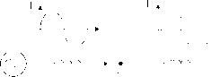

AC Mains

system

coupling

Compensation current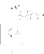

Act! e Filter

FIGURE 33.2 Compensation characteristics of a shunt active power fiher.

system sees the non-linear load and the active power filter as an ideal resistor. The compensation characteristics of the shunt active power filter is shown in Fig. 33.2.

33.3.1 Power Circuit Topologies

Shunt active power filters are normally implemented with PWM voltage-source inverters. In this type of application, the PWM-VSI operates as a current-controUed voltage-source. Traditionally, 2 levels PWM-VSI have been used to implement such system connected to the ac bus through a transformer. This type of configuration is aimed to compensate nonlinear load rated in the medium power range (hundreds of kVA) due to semiconductors rated values limitations. Fiowever, in the last years multUevel PWM voltage-source inverters have been proposed to develop active power filters for medium voltage and higher rated power applications. Also, active power filters implemented with multiples of VSI connected in paraUel to a dc bus but in series through a transformer or in cascade have been proposed in the technical literature. The different power circuit topologies are shown in Fig. 33.3.

The use of VSI connected in cascade is an interesting alternative to compensate high power nonhnear loads. The use of two PWM-VSI with different rated power aUows the use of different switching frequencies, reducing switching stresses and commutation losses in the overaU compensation system. The power circuit configuration of such a system is shown in Fig. 33.4.

on inear oad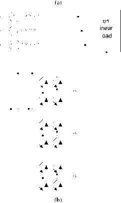

FIGURE 33.3 Shunt active power fiher topologies implemented with PWM voltage-source inverters, (a) A three-phase PWM unit, (b) Three single-phase units in parallel to a common dc bus.

The voltage-source inverter connected closer to the load compensates for the displacement power factor and lower frequency current harmonic components (Fig. 33.5(b)), while the second compensates only high frequency current harmonic components. The first converter requires higher rated power than the second and can operate at lower switching frequency. The compensation characteristics of the cascade shunt active power filter is shown in Fig. 33.5.

In recent years, there has been an increasing interest in using multUevel inverters for high power energy conversion, specially for drives and reactive power compensation. The

AC ource

ink Inductor rv-v-v-v

rY-Y-Y-> (TV.

rYrV-> its-

Current Reference Generator

Gating ignals Generator

Current Control ystem

oltage Control

DC oltage Reference

ink Inductor

Current Reference Generator

Г

Gating ignals Generator

Current Control ystem

on inear oad

oltage Control

DC oltage Reference

FIGURE 33.4 A shunt active power filter implemented with two PWM VSI connected in cascade.

use of neutral-point-clamped (NPC) inverters (Fig. 33.6) allows equal voltage shearing of the series connected semiconductors in each phase. Basically, multilevel inverters have been developed for apphcations in medium voltage ac motor drives and static var compensation. For these types of applications, the output voltage of the multilevel inverter must be able to generate an almost sinusoidal output current. In order to generate a near sinusoidal output current, the output voltage should not contain low frequency harmonic components.

However, for active power filter applications the three level NPC inverter output voltage must be able to generate an output current that follows the respective reference current containing the harmonic and reactive component required by the load. Currents and voltage waveforms obtained for a shunt active power filter implemented with a three-level NPC-VSI are shown in Fig. 33.7.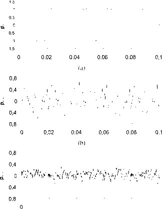

0,02 0,04 0,06 0,08 0,1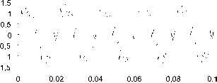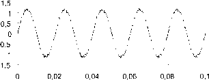

FIGURE 33.5 Current and voltage waveforms of active power filter implemented with two PWM VSI in cascade, (a) Load current waveform, (b) Current waveform generated by PWM VSI #1. (c) Current waveform generated by PWM VSI #2. (d) Power system current waveform between the two inverters (THDi = 13.7%). (e) Power system current waveform (THDi = 4.5%).