Computer Simulation of Power Electronics and Motor Drives

Michael Giesselmann, Ph.D., P. E.

Department of Electrical Engineering Texas Tech University Lubbock, Texas 79409, USA

34.1 Introduction...................................................................................... 853

34.2 Use of Simulation Tools for Design and Analysis..................................... 853

34.3 Simulation of Power Electronics Circuits with PSpice®............................ 854

34.4 Simulations of Power Electronic Circuits and Electric Machines................. 857

34.5 Simulations of ac Induction Machines using Field Oriented (Vector)

Control............................................................................................. 860

34.6 Simulation of Sensorless Vector Control Using PSpice® Release 9.............. 863

34.7 Simulations Using Simplorer®.............................................................. 868

34.8 Conclusions....................................................................................... 870

References......................................................................................... 870

34.1 Introduction

This chapter shows how power electronics circuits, electric motors and drives, can be simulated with modern simulation programs. The main focus wiU be on PSpice®, which is one of the most widely used general-purpose simulation programs and Simplorer®, Release 4.1, which is more specialized towards the power electronics and motor drives apphcation area. Ali Ricardo Buendia, who is currently working towards his MSEE degree, has created the examples for Simplorer®. The PSpice® examples have originally been developed for Release 8 from MicroSim and have been converted to the current Release 9. Examples for both versions are given. The examples in this chapter have been chosen such that they can be run on the evaluation versions of the particular programs. The author found this to be very beneficial in an educational environment, since such examples can be shared with students to enhance their understanding of the lecture material. This shaU by no means lead to the conclusion that the programs and simulations presented here cannot be used for serious professional work. In fact, the author has used these tools with great success in many research and consulting projects. In addition to the programs mentioned above, MathCAD® has been used to derive and present the underlying equations. The advantage of using MathCAD® for this purpose is, that in

MathCAD® it is possible to check equations by actually executing them.

The examples have been developed to iUustrate advanced techniques for simulation of systems from the power electronics and drives area but not to teach the basic features of the individual programs. It is assumed, that the reader wiU famUiarize themselves with the basics on how to run the programs using the accompanying documentation. In addition, it is assumed that the reader is famUiar with the basics of power electronics and electric machines, specifically ac induction machines. For a review the reader shaU be referred to [2] for power electronics and [3,7] for induction machines.

34.2 Use of Simulation Tools for Design and Analysis

Before any in-depth discussion of specific simulation examples, it is appropriate to reflect upon the value of simulations and its place in the design and analysis process. Computer simulations enable engineers to study the behavior of complex and powerful systems without actually buUding or operating them. Simulations therefore have a place in the analysis of existing equipment as weU as the design of new systems. In addition, computer simulations enable engineers to safely

study abnormal operating or fault conditions without actually creating such conditions in the real equipment.

However, the reader should be reminded that, even the most modern simulation programs cannot perfectly represent all parameters and aspects of real equipment. The accuracy of the simulation results depends on the accuracy of the component models and the proper identification and inclusion of parasitic circuit elements such as parasitic inductance, capacitance and parasitic mutual couphng. Accuracy of component models in this context shall not mean that the model is actually faulty but rather that the limitations of the model are exceeded. For example, if the transformer inrush phenomenon were to be studied using a linear model for a transformer, the simulation would not yield useful results.

In particular, the precise prediction of voltage and current traces during fast switching transitions in power electronics circuits has been proven to be difficult. To obtain useful results, extensive experimental validation, advanced device models (and the values for their parameters!) and detailed knowledge of parasitic elements, including those of the packaging of the circuit elements, are necessary. In addition, numerical convergence is often a problem, if gate drive signals, with rise and fall times as steep as in real circuits, are applied. Therefore, the exact prediction of waveforms during switching transitions shall be excluded from the discussions in this chapter. Consequently, the author prefers to measure parameters such as voltage rise and fall times, over and undershoot, etc., on actual circuitry in the laboratory.

Sometimes, users of PSpice® claim that the convergence problems are so severe that its use for simulations of power electronics circuits is just not possible or worth the effort. However, this is absolutely not true and with the proper techniques of gate signal generation, we can simulate just about any given circuit with little or no convergence problems. In addition, if convergence problems are avoided, simulations run much faster and larger numbers of individual transitions can be studied. This is achieved by generating gate signals that are slightly less steep than in real circuits using analog behavioral elements. This gives a lot of insight into the cycle by cycle as well as the system level behavior of a power electronics circuit. In this fashion, the function of an existing, as well as the expected performance of a new, proposed circuit, can be studied. An excellent application for these cycle-by-cycle simulations is the development and verification of control strategies for the power semiconductors.

Analog behavioral modehng (ABM) techniques included in PSpice® can be used to study large and complex systems like the control of induction machines using field oriented (also called vector) control techniques. Examples are given that replace the power electronics inverter with an ABM source that produces voltages, which represent the short term average (filtering away the voltage components of the switching frequency and above) of the output of a three-phase inverter. These examples represent pure system level simulations, which

could have also been done using programs like MatLab/Simulink®. However, circuit simulation programs provide the option of studying actual circuit level details in complex systems. To demonstrate this capability, the startup of an induction motor, fed by a three-phase MOSFET inverter, is presented.

In all modehng cases, the user needs to define the goal of the simulation effort. In other words, the user must answer the question What information shall be obtained through the simulation of the circuit or system? The user must then select the appropriate simulation software and the appropriate models. This process requires a detailed understanding of the properties and limitations of the device models and the sensitivity of the results to the model limitations. In order to obtain such an understanding, it is often recommended and necessary to perform numerous simulation test runs, carefully scrutinize the results and compare them with measured data, results from other simulation packages or otherwise known facts.

34.3 Simulation of Power Electronics Circuits with PSpice®

The first example of a power electronics circuit is a step-down (also called Buck) converter with synchronous rectification. For the purpose of synchronous rectification, the diode, which connects the inductor to ground in the regular circuit, is replaced with a power MOSFET transistor. The benefit of this circuit is, that the power MOSFET represents a purely resistive channel in the on state. This channel does not have a residual, current independent, voltage drop like the p-n junction of a diode. Therefore, the voltage drop across the MOSFET can be made lower than what can be achieved with diodes. The results are reduced losses and increased efficiency. To achieve this, the lower MOSFET must be turned on whenever the upper MOSFET is turned off and the current in the inductor is positive. If the current in the inductor is continuous, the drive signal for the lower MOSFET is simply the inverted drive signal for the upper MOSFET. However, if the current in the inductor is discontinuous, the drive signal for the lower MOSFET must be cut off as soon as the current in the inductor goes to zero. Figure 34.1 shows a simulation setup for a synchronous buck converter that can operate correctly for continuous as well as discontinuous inductor current.

As mentioned before, the key element of this example is the circuit for the generation of the gate drive signals for the MOSFETs. For clarity this circuit has been realized using only standard elements from the libraries of the evaluation version. The basic principle of the operation of the gate drive circuit is the well-known carrier based scheme, where a control voltage is compared with a triangular carrier with fixed amplitude. An ABM block, shown in the lower left part of Fig. 34.1, generates the triangular carrier. Eqn. (34.1) below gives the

PARAMETERS:

.17РГ) Acos(Cos( 2*Pi*Fsw*Time + Pi/2))

Triangle

EVALUE IF(V(%IN+)>2, V(%IN+),0)

0 2-

EVALUE

IF(V(%IN+)<-2, IF(V(%IN-)>40m, -V(%IN+),0),0)

FIGURE 34.1 Simulation setup for a synchronous Buck converter.

equation for the triangular carrier wave. The output range of the function shown in Eqn. (34.1) is between 0.0 and 1.0.

Erri(t) := acos(cos(2f3t +1)) (34.1)

For the generation of the gate drive signals, the carrier wave is compared with a control signal that can have values between 0.0 and 1.0, corresponding to a duty cycle input between 0% and 10%. Feeding the difference of the carrier wave and the control signal into a soft comparator generates the primary PWM signal. Careful inspection of the implementation of the soft-limiter element provided in the evaluation version of PSpice® shows, that it uses a scaled hyperbohc tangent function. Figure 34.2 shows a plot of a hyperbohc tangent function. It can easily be seen that the result of the soft limiter is an output signal with smooth transitions, which is crucial to avoid convergence problems in PSpice®. The soft hmiter used

here has an upper and lower limit of ±15 V and a gain (steepness control for the tanh function) of 1000 (Ik).

Figure 34.3 shows the output of the simulation run for the synchronous buck converter. The top-level graph shows the generated triangle carrier. It has a frequency (Fsw, see parameter statement in Fig. 34.1) of 10 kFiz. This frequency has been chosen rather low to improve the readability of Fig. 34.3. In the graph below the triangle voltage in Fig. 34.3, the gate drive signals are shown for both MOSFET transistors. Please note that the gate drive signal for the lower MOSFET is vertically shifted by 30 V in order to separate the traces for readability. The graph below the gate drive signals shows the inductor current. It can be seen that the current is discontinuous after the initial inrush peak. The inrush peak is caused by the fact that the capacitor is initially discharged (1С = 0 V). It is evident, that the gate drive signal of the lower (synchronous rectification) MOSFET is appropriate for the inductor current. The bottom trace shows the capacitor voltage, with has a steady state value of slightly more than 0.5x40V (0.5 = 50%) being the duty cycle and 40 V being the input voltage) due to the fact that the inductor current is shghtly discontinuous even at steady-state conditions. To test the gate drive circuit for the lower MOSFET, the load has been chosen such that the steady-state current would be discontinuous. FoUowing the soft hmiter are two voltage-controlled voltage sources that generate isolated gate-source vohages of 15 V for the on condition and OV for the off condition of the MOSFETs. To enable operation with discontinuous inductor current, the source E- in Fig. 34.1 also monitors the polarity of the inductor current through a current controlled voltage source Fil with unity gain.

In addition to the cycle-by-cycle simulation of a dc-dc converter, it is also possible to use a time-averaged replacement for the MOSFET transistors used in the circuit in Fig. 34.1. In fact, a common time average model can be used for the Buck, the Boost, the Buck-Boost, and the Cuk converter as long as they operate with continuous inductor current. The time-averaged model has the advantage that it can run much

tri angle voltage

. U(Tt-iangle)

LJliLmU

1ШШи1ШШШ1]ШШШШШШ

FIGURE 34.2 Plot of a hyperbolic tangent function used to generate smooth PWM signals.

FIGURE 34.3 Output waveforms for the synchronous buck converter.

faster since it does not have to follow each switching transition. It is also possible to perform dc and ac sweep analyses. A dc sweep would sweep the duty cycle over a wide range and show the output voltage as a function of the duty cycle. An ac sweep analysis would sweep the frequency of an ac signal, that is superimposed on top of the duty cycle bias signal. The ac sweep allows the study of the behavior of the converter, including a feedback control system, in the frequency domain for traditional stability analysis and system tuning. A detailed description of this time-averaged modeling technique, including detailed examples is given in [1].

To illustrate the capabilities of the PSpice® simulation program, the next example shows a complete three-phase inverter bridge using six power MOSFETs. This circuit is shown in Fig. 34.4. Note that free-wheeling diodes are an integral part of every power MOSFET and are not shown separately. The inverter drives a three-phase load, which could represent an induction motor for a singular operating point. The load is connected to the inverter output terminals with so-called connection bubbles. Due to the number of elements involved, the circuit for the gate drive signal generation is contained in a hierarchical block. Blocks like this are available from the main toolbar in the schematic editor. Double chcking on this block called PWM Generator reveals the subcircuit which is shown in Fig. 34.5.

The hexagonal shaped symbols named 1+ , 1- , 2+ , etc., are called interface ports. These interface ports provide the connection between the subcircuit and the ports of the hierarchical block above. Here the connection is to the ports (dots) on the PWM Generator block. The interface ports are created by simply drawing a wire up to the boundary of the block. The name of the port is initially generic, Px , where x is a running number, but can be easily edited by double-chcking on the generic name. After drawing a block and creating all the ports, double-chcking inside the box will open up a schematic page for the subcircuit which has all the appropriately named interface ports already in it. Additional details on hierarchical techniques can be found in [10].

PWM Generator

150V . Vbus+

150V Vbus-

RARAMETERS: m a 0.8 AC amp {m a}

RARAMETERS:

AC freq 60

FsW 3.6k

Ri 3.1415Э265

25 150mH

RJoad b LJoad b

25 150mH

R loa(J c L loacl c

3-Phase SPWM Generator:

Level Shifter and Driver

E a+

VAMPLHAC amp} FREQ={AC fTeq} PHASE=0 -

о

l+)>2.0,

IF(V(%IN+): E

V(%IN+),0)

VAMPL={AC amp} FREQ={AC fTeq} PHASE-12D

VAMPL={AC amp} FREQ={Ac fTeq} PHASE=+10

(27Fif

IF[V(%IN+) E b+

>t<-2-V(%IN+),0)

о

IF(V(%IN+)>2.0, V(%IN+),0) E b-

EVALUE IFCV(%IN+)<-2.0,-V(%IN+),0)

E c+

о

+15-500 IS

PWMc

EWLUE IF(V(%IN+)>2.0, V(%IN+),0)

E c-

IF(V(%IN+)-

, -V(%IN+),0)

Vtriangle

FIGURE 34.5 PWM generation sub-circuit for a three-phase MOSFET inverter.

The circuit shown in Fig. 34.5 is similar to the gate-drive generation circuit discussed before. Circuits like the circuit shown in Fig. 34.1 compare a triangular carrier with one or more reference signals. In this case, three reference signals, one for each phase, are used. The triangular carrier signal is symmetrical with respect to the time axis. The values cover the range from -1.0 to 1.0. The equation for the carrier signal is given by Eq. (34.2):

Erri(t) := asin(sin(2f3t + )). (34.2)

The three reference signals are sinusoidal signals with equal amplitude and a relative phase shift of 120°. For linear modulation, the amplitude range of the reference signals is hmited to the amplitude of the triangular carrier, e.g. 1V. The ratio of the reference wave amplitude and the (fixed) carrier amplitude is called amplitude modulation ratio m a . In the circuit shown in Fig. 34.4 m a has a value of 0.8. This value is defined by a parameter symbol and represents a global parameter, which is visible throughout all levels of the hierarchy. The phase to neutral voltage amplitude of each inverter leg is equal to Vbus + (shown in Fig. 34.4) multiplied with the amplitude modulation ratio. The frequency and waveshape of the phase to neutral voltage of each phase leg is equal to the reference waveform, if the high frequency components resulting from the carrier wave are filtered away. This way, each inverter leg can be viewed as a linear power amphfier for its reference voltage. In fact, in drive applications, inverters are often called servo-amphfiers . The load typically reacts only to the low-frequency components of the inverter output voltage. The high-frequency components, which include the triangular carrier frequency (also called switching frequency)

and its harmonics, are typicaUy just a blur for the load. This is especially true in recent times, where switching frequencies of 20 kHz and above are common. As an added benefit, audible noise is avoided at these frequency levels.

The circuit involving the soft limiter and level shifter/high side driver in Fig. 34.5 is very simUar to the circuit for the synchronous buck converter, except for the fact that the load current is not monitored. The control functions for the E x+, E x- sources, where x denotes the phase, are chosen such that the activation voltage levels are ±2 V. If the output voltage of the soft-limiter is between -2 V and +2V, no MOSFET is activated, and shoot-through, meaning a short-circuit between the positive and negative bus, is avoided.

Figure 34.6 shows the simulation results for the three-phase inverter. The time scale is slightly stretched to show the detaUs of the PWM signals better. The graph on top represents the line-to-line voltage Vg. The graph below shows the load currents for aU three phases. Due to the inductors contained in the load, the current cannot instantaneously change and foUow the PWM signal. Therefore the load current is an almost pure sinusoid with very little ripple. This is representative of the hne currents in induction motors.

Figure 34.7 shows that the MOSFETs in Fig. 34.4 can be replaced with IGBTs. The particular IGBT shown here is included in the library of the evaluation version. Note that free wheehng diodes are needed, if IGBTs are used. The free wheehng diodes carry the load current when the IGBTs are turned off to provide a continuous path for the current. This is very important, since the load can have a substantial inductive component. Whenever the diodes are conducting, energy flows momentarily back to the source. In the case of power MOSFETs, the diodes (often called body diodes) are an integral part of the device. In the symbol graphic of PSpice® these body diodes are not shown for MOSFETs. For this circuit, the gate drive circuit and the results are the same as for the three-phase bridge with power MOSFETs.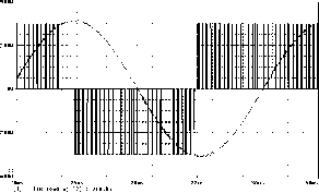

PWM Generator

2+ 150V jj IGBTllr # 2 i+0- Л

IGBT3 [ jXGH40NG0

PARAMETERS: AC amp {m a}

PARAMETERS:

ACfreq 60-

Fsw 3.6k

Pi 3.14159265

25 15DmH

RJoacl b LJoad b

FIGURE 34.6 Output waveforms of the three-phase inverter with MOSFETs.

FIGURE 34.7 Three-phase inverter circuit with IGBTs.

34.4 Simulations of Power Electronic Circuits and Electric Machines

In the foUowing, the startup of an induction motor, fed by the three-phase inverter shown in Fig. 34.4, is shown. For this purpose, the simple passive load in Fig. 34.4 is replaced by an induction motor. For this and further discussions it is assumed that the reader is famUiar with the theory of induction machines. A number of exceUent references are given at the end of this chapter [3,4,5,7]. The induction motor symbol represents the electromechanical model of an induction motor. The model is suitable for studies of electrical and mechanical transients as weU as steady state conditions. The output pin on the motor shaft represents the mechanical output. The voltage on this pin represents the mechanical angular velocity using the relation 1 V = 1 rad/s. In addition, any current drawn from or fed into this terminal represents applied motor or generator torque according to the relation 1 A = 1 Nm. Due to these definitions, the electrical power associated with the voltage of the motor shaft (with respect to ground) is identical to the mechanical power. FoUowing the weU-known theory, the induction motor model has been derived for a two-phase (direct and quadrature, D, Q) equivalent motor. Attached to the motor is a bi-directional two-phase to three-phase converter module. This module is voltage and current invariant. This means that the voltage and current levels in the two-phase and the three-phase machine are equal. Consequently, the power in the two-phase machine is only of the power in the three-phase circuit. This is accounted for in the calculation of the electromagnetic torque (see Eq. 34.4 below). The internally generated torque can be monitored on the output labeled Torque on top of the sleeve around the motor shaft. The linear load in Fig. 34.8 is a symbol that represents an appropriately sized resistor to ground.

In Fig. 34.8 the motor is represented by a custom symbol caUed Motor 1 . A simple hierarchical block could have been used for the motor, but a custom symbol has been created to

pwm generator

3+ 3+ 3- -эз-

5+ 5+ 0 5-

200v vbus-

irf1

® irf1

200v vbus-

irf1

parameters: freq ac 60 omega {2*pi*freq ac} pi 3.14159265

r sense a

r sense b -wv-h

r sense 1ж

FIGURE 34.8 Induction motor startup with three-phase inverter circuit.

achieve a more reahstic and pleasing graphical representation. The symbol can be easily created with the symbol editor, which is build into the regular schematics editor. The editor provides standard graphical elements (hues, rectangles, circles) etc., so that professional looking symbols can easily be created. More details on this are shown below in Figs. 34.19, 20 and the accompanying discussion. The motor symbol resides in a local library (.sib), which is located in the same subdirectory, where all other files for the project are residing. The library is configured (the simulator is told of its existence) by using the menu dialog Options/Editor Configuration/Library Settings/Add Local . These parameters are passed onto the subcircuit by using the name of the parameter preceded by a symbol. The advantage of passing parameters to sub-circuits in this way is that several symbols can call one set of subcircuits with different parameters (Table 34.1).

Double-clicking on the motor symbol reveals the associated subcircuit that implements its function. This sub-circuit is

TABLE 34.1 List of aU attributes used for the induction motor symbol

Attributes

PART = Induction Servo MODEL = Ind Motor TEMPLATE = J mot = 0.01 Omega init = 0.0 Ls = (@Lm + @Lsl) Lr = (@Lm + @Lrl) Poles = 4

Tau r = (@Lr/@R Rot) REFDES = Motor? Lsl= 14.96 mH Lrl = 8.79mH R Stat = 3.60 R Rot = 1.90 Lm = 424.4 ImH

shown in Fig. 34.9. The upper portion of this subcircuit represents the electrical model. The task of the electrical model is to calculate the stator and rotor currents, where the stator voltages and the mechanical speed of the machine are input parameters. However, it is also possible, without any changes, to feed stator currents (with controlled current sources) into the D and Q inputs and have the model calculate the appropriate stator voltages. This option is useful for vector control applications, which are discussed later.

The equation system for the electrical model is given by Eqn. (34.3): The theory for this equation system is derived in [3,4,5,7]. The equation system and the model are formulated for the stationary reference frame. This reference frame assumes that the frame of the machine is stationary (which is hopefully the case in the real machine!) and the voltages and currents of the rotor are equivalent ac values with stator frequency. From machine theory we know that the actual rotor currents have slip frequency. Another reference frame is the synchronous (also called excitation) reference frame. In this reference frame the stator of a fictitious machine is assumed to rotate with synchronous speed. The advantage of this reference frame is that the input frequency is zero (dc), which makes it easy to explain the principle of vector control by extending the theory of dc machines to ac machines.

L,=L L3I Lr = + 4l

p=Jt

(34.3)

Sometimes still other reference frames are used and it is possible to generate a universal electrical model with a reference frame speed input. This model could then be used for any reference frame.

The electrical model shown in Fig. 34.9 implements the equation system Eqn. (34.3). The circuit closely resembles the well-known T equivalent circuit for the steady state analysis of induction machines. Two instances of the T equivalent circuit are necessary to implement the two-phase (D, Q) model. The two instances of the circuit are almost mirror images of each other (and actually drawn that way) except for some differences in the circuit elements that calculate the voltages, which are generated due to the rotation of the rotor. The bottom of Fig. 34.9 represents the mechanical model. This circuitry calculates the internally generated electro-magnetic torque

Electrical Model:

Rs q

<CQI>-ЛЛЛ

j-sl q

{@R Stat} Hsq @lsI} {1.5@Lm@Poles/2}

Lrl d Lmag d

Lmag q

SR Rot}

-ли-(xV

Rr d

(-)4v(%IN1 *@Lm +V(%IN2)

Rotational Voltages: tV(%IN1

{@Lrl} Hrq

Mechanical Model:

Rot}

rd o{V Lsd -1

J rnot} I orque

Omega tnech

{@Poles/2}

H Load GAIN=1

FIGURE 34.9 Subcircuit for induction motor model.

using the rotor and stator currents as input values. The equation for the torque is given by Eqn. 34.4 [3,4,5,7]:

T = --LWr-W-

(34.4)

side. The equation system for this voltage and current invariant transformation is given by Eqn. (34.5). This transformation is sometimes caUed Clark or ABC-DQ transformation. Note that Vq denotes a zero-sequence voltage, which is assumed to be zero. This voltage would only have non-zero values for unbalanced conditions. An interesting detail of the subcircuit is the three-phase switch on the input. This switch is necessary to ensure a stable initiahzation of the simulator in case the machine is fed with a controUed current source. The switch provides an initial shunt resistor from the three-phase input to ground. Soon after the simulation has started, the switch opens and leaves only a negligible shunt conductance to ground.

2 -1 -1

0 V3 -V3 11 1

2 0 2

-1 V3 2 -1 -V 2

(34.5)

The factor accounts for the fact that the real motor is a three-phase machine. Using the generated torque, the load torque and the moment of inertia, the angular acceleration can be calculated. Integration of the angular acceleration yields the rotor speed, which is used in the electrical model. To avoid clutter and to improve readability, connection bubbles are used to connect the various parts of the model together.

Since typical induction machines are three-phase machines, it is often desirable to have a machine model with a three-phase input. Therefore a bidirectional two-phase to three-phase converter module, which can be attached to the motor, has been developed. A subcircuit for this module is shown in Fig. 34.10. This circuit is truly bidirectional, meaning that the circuit can be fed with voltage or current sources from either

Figure 34.11 shows the result for the startup of the induction motor for the circuit of Fig. 34.8. The motor is a 1/2 hp, 208 V, 4-pole machine. The detaUed parameters are shown in Table 34.1. The PWM generation was identical to the example shown in Fig. 34.4, except that the switching frequency was 4 kFiz and 21.1% of the third harmonic has been added to each of the reference sinusoids in order to increase the linear modulation range. The resulting reference waveform was then multiplied with 1.14, which represented the maximum voltage for linear modulation. The top trace in Fig. 34.11 shows the developed electromagnetic torque, the zero level and the level for the rated steady-state torque (2 Nm). This graph shows the typical osciUatory torque production of the induction machine for uncontroUed line start. The scale for this

Ron=500 Roff=50k Toff=1ms

ABC <-> DQ Transformation:

V(%IN)

-V(%IN1)/2 Ф +sqrt(3) V(%IN2)/2

-V(%IN1)/2

-sqrt(3) *V(%IN2)/2

(V(%IN1) -V(%IN2)/2 -V(%IN3)/2) *2/3

(V(%IN1) -V(%IN2)) /SQRT(3)

Simulation Startup Support for Current Source Drive

GAIN=1

H d H q

<ZDI>

GAIN=1

FIGURE 34.10 Subcircuit for the ABC-DQ transformation module.

i0i----------------------------------------------------------

□ U(Motor1:Torque Monitor) * 2 v В 2вви-г----------------------------------------------------------

Rotor Speed/ IV = Irad/sec eu ------------------------------------------------------------------------------------

□ U(Motor1:0nech)

JtOfi-r--------------------------------------------------------------------------------------

-JtOfl---------------------------------------------------------------------------------------

□ I(R sense a) * I(R sense b) v I(R sense c) 5вви-г

SEL i -5вви+-

es 50ns 100ms 150ms 2e0ms 250ms 300ms

□ U(fl,B)

Time

FIGURE 34.11 Induction motor startup with three phase inverter circuit.

graph is 1V = 1 Nm. The graph below shows the mechanical angular velocity with a scale of 1 V = 1 rad/s. Below the graph for the rotor speed, all three input currents are shown. It is evident that the current traces are almost perfect sinusoids, despite the fact that the input voltage is the PWM waveform shown in the bottom graph. Also, the trace for the torque shows no discernable high-frequency ripple. The reason is of course, that the motor windings are inductive, and represent a low pass filter for the applied voltages. Nevertheless, recent research suggests that filtering the output voltage of the inverter is advantageous anyway, because it significantly reduces the voltage stress on the windings and suppresses displacement currents through the bearings [8].

34.5 Simulations of ac Induction Machines using Field Oriented (Vector) Control

The following examples will demonstrate the use of PSpice® for simulations of ac induction machines using Field Oriented Control (FOC). Again, it is assumed that the reader is familiar with the basics of induction machine theory. Often times FOC is also called vector control, and both expressions can be used interchangeably. Field oriented control was proposed in the 1960s by Hasse and Blaschke, working at the Technical University of Darmstadt [6]. The basic idea of field oriented control is to inject currents into the stator of an induction machine such that the magnetic flux level and the production of electromagnetic torque can be independently controlled and the dynamics of the machine resembles that of a separately excited dc machine without armature reaction. The previously discussed two-phase model for the induction machine is very helpful for studies of vector control and shall be used in all examples. If a two-phase induction motor model for the synchronous (or excitation) reference frame is used, the similarities between the control of a separately excited dc machine and vector control of an ac induction machine would be most evident. In this case, the D input would correspond to the field excitation input of the dc machine and both inputs would be fed with dc current. Assuming unsaturated machines, the current into the D input of the induction machine or the field current in the dc machine would control the flux level. The Q input of the induction machine would correspond to the armature winding input of the dc machine and again both inputs would receive dc current. These currents would directly control the production of electromagnetic torque with a linear relation (constant k) between the current level and the torque level. Furthermore, the Q component of the current would not change the flux level established by the D component. To make such a simulation work, it would finally be necessary to calculate the slip value that corresponds to the commanded torque and

supply this dc value to the D,Q (synchronous reference frame) machine model.

Of course this is very interesting from an academic standpoint and the author uses this example in a semester long lecture on field oriented control. However, it should again be noted that a machine represented by a model with a synchronous reference frame would have a stator, which rotates with synchronous speed. Of course this is not realistic and therefore it is more interesting to generate a simulation example that uses the previously discussed motor with a model for the stationary reference frame. This motor must be supphed with ac voltages and currents with a frequency determined mostly by the rotor speed to a small extent by the commanded torque. We still supply dc values representing the commanded flux and torque but we transform these dc values to appropriate ac values. In the following example we will assume that we can measure the actual rotor speed with a sensor. This can in effect be easily accomplished and many types of sensors are available on the market. If we add the slip speed, that we determine mathematically from the torque command, to the measured rotor speed, we obtain the synchronous speed for the given operating point. With this synchronous speed we can transform the dc flux and torque command values from the synchronous reference frame to the stationary reference frame. We accomplish this by using a rotational transformation according to the matrix equations in Eqn. (34.6). This rotational transformation is also called Park transformation:

Dout

cos(p) - sin(p)

.%utJ Lsin(p) COs(p) JLQin

Dout

cos(p) sin(p)

Qout J L - sin(p) cos(p) J L Vqin

cos(p) - sin(p)

sin(p) cos(p) J [ - sin(p) cos(p)

cos(p) sin(p)

1 0 0 1

(34.6)

As shown in Eqn. (34.6), the transformation is bidirectional and the product of the transformation matrices yields the unity matrix. For the following discussion we shall define the transformation, which produces ac values from dc inputs as a positive vector transformation and the reverse operation as consequently a negative vector transformation. The matrix equation for the positive vector transformation is shown on the left-hand side of Eqn. (34.6). The negative transformation is very useful to extract dc values from ac voltages and currents for diagnostic purposes. We will also make use of it for sensorless vector control, which is discussed below. Both rotational transformations use the angle, p, in the equations. This angle can be interpreted as the momentary rotational displacement angle between two Cartesian coordinate systems; one containing the input values and the other one the output values. This angle is obtained by integration of the angular

Indirect Vector Control of an Induction Motor:

Omega mech

Torque

>Flux офО A<)-\ ОфО

Vector Controller >Omech

QOQ C<->C QOQ

JV Flux V

Torque

PARAMETERS: V LL 203

PARAMETERS: Freq n

V ph pk {Sqrt(2rV LUsqrt(3)} Omega n {2*Pi*Freq n} Psi n {V ph pk/Omega n} Pi 3.14159265

Ratio=0.5 830 RPI

FIGURE 34.12 Top level circuit for indirect vector control of induction motors.

velocity with which the coordinate systems are rotating (typically the synchronous speed).

In summary, we replaced a theoretical motor model using a synchronous reference frame by a reference frame transformation of the supply voltages and currents. In fact, there are integrated circuits on the market like the ADMC-200 from Analog Devices, which is optimized to perform both the Clark and the Park transformation in both directions [ 1 ].

Figure 34.12 shows the top level of a simulation example that implements vector control for an induction machine with a stationary reference frame model. In fact, the motor model and the associated sub-circuits are identical to the ones used for the circuit shown in Fig. 34.8. Fiowever, a more powerful motor is used here, specifically a 3 hp, 4-pole 208 V motor with circuit parameters shown in Table 34.2. As discussed above, the actual speed of the rotor is used as an input signal for the control unit. This scheme is known as indirect vector control and represents one of the most often used arrangements. The symbol for the controUer has the same parameters as the motor. This is necessary to achieve correct field orientation. In real systems, the controUer also must know

TABLE 34.2 List of all attributes for the induction motor symbol for vector control

Attributes

PART = Induction Servo MODEL = Ind Motor TEMPLATE = J mot = 0.1 Omega init = 0.0 Ls = (@Lm + @Lsl) Lr= (@Lm + @Lrl) Poles = 4

Tau r = (@Lr/@R Rot) REFDES = Motor? Lsl = 2.18mH Lrl = 2.89mH R Stat = 0.48 R Rot = 0.358 Lm = 51.25mH

or somehow determine the machine parameters. The machine parameters could have also been established globally using PARAM symbols, but if the parameters for the controUer can be set separately as is the case here, the influence of parameter mismatch on the performance of the control can be easily studied. An example of this is given below.

Figure 34.12 also shows a symbol for a mechanical gear, which is attached to the output of the induction motor. Let us recaU that the voltage on the mechanical output terminal represents the angular velocity and the current represents the torque. We also know that the product of the angular velocity and the torque is the mechanical power. Therefore it is easily understood that the electrical representation of an ideal gear is an ideal transformer. The ideal transformer changes speed (voltage) and torque (current) just like an ideal gear. Also there are no power losses in an ideal transformer as weU as in an ideal gear.

In this fashion, many more mechanical properties and devices can be modeled. For example, a mechanical flywheel is simply represented by a capacitor to ground. Due to the scaling factors for the angular velocity and the torque, a flywheel with / = 1 kg m would be a capacitor with С = 1 F. The comphance of a drive-shaft (elastic twisting by the applied torque) can be modeled by a series inductor. By including both capacitors and inductors, effects like mechanical resonance can be included in a model.

Figure 34.13 shows the subcircuit for the vector control unit. The central part is a vector rotator for positive direction. This element transforms the dc reference values for the flux (D axis) and the torque (Q axis) to the stationary reference frame. The input angle for the vector rotator is the integral of the synchronous angular velocity. The signal caUed Omega o is the measured rotor speed.

This speed is multiplied with the number of pole-pairs (poles/2) to obtain the electrical angular velocity. Then the slip value (see Eqn. (34.7)) appropriate to the torque command is added and the resulting signal is routed through an integrator to generate the input angle for the vector rotator.

In the D axis, a differentiator function DDT() is used in a compensation (see Eqn. (34.8)) element which assures that the actual flux in the machine foUows the commanded signal

Controller for Indirect Vector Control:

{1/@Lm}

<¥Ш>-r

Torque

/(%IN1) \J(@kT*V(%IN2)

{@Poles/2}

V(%IN)H DDT(V(%IN)r @Tau г

OrTieg o

>ln D -Out D

Vec Rot

V(%IN)

V(%IN)

FIGURE 34.13 Sub-circuit for indirect vector control of induction motors.

without delay. The input and output values of the vector rotator are voltage signals which correspond 1:1 to current signals. (In a real controller the currents are typically scaled values in the memory of a digital signal processor, DSP.) In fact, the vector controller calculates the appropriate currents that need to be injected into the machine to perform as desired. Two voltage-controlled current sources with unity gain are connected to the output of the vector rotator to generate these currents. In a real system, the controlled current sources are realized by an inverter with current feedback. In the most reahstic case, this would be a three-phase inverter and the ABC-DQ transformation would be performed before the current-controlled inverter. In this example, the ABC-DQ transformation has been performed outside the controller and outside the motor. This way, it is possible to study vector control principles using a DQ controller and a DQ motor by ehminating the ABC-DQ transformation elements. An example is given in Fig. 34.14.

slip

4d =

(rd + AdP)

(Trrd)

1+TrP

d Jt

(34.7) (34.8)

Figure 34.15 shows the results obtained for the circuit shown in Figs. 34.12-34.14 with perfect tuning of the vector controller, meaning that the controller precisely knows all

motor parameters. The two traces in the diagram on top of Fig. 34.15 represent the traces for the D and Q input signals of the vector rotator. The graph below shows the reference value for the flux. It is evident that the flux level is being changed at the same time when 10 Nm of torque is commanded (and produced). This is done to check if the torque and the flux can be independently controlled, which is true for correct field oriented control. Below the flux reference is the graph for the mechanical angular velocity. It can be seen that the machine accelerates whenever torque is developed and slows down due to the load when the torque command is driven to zero. The graph on the bottom of Fig. 34.15 provides the easiest way to judge the quality of the correct field orientation. This graph shows the traces of the commanded and the actually produced torque and in this case they are perfectly on top of each other at all times.

Figure 34.16 is an example of the results obtained from a detuned vector controller. The circuit is identical to the circuit in Fig. 34.12, except for the fact that the rotor resistance value in the controller was increased to 125%. It is obvious that the traces for the commanded and the actually produced torque are no longer identical. This is especially true during times when the flux is changing. Detuning is actually a real problem in industrial vector control applications. Detuning is caused by the fact that the machine parameters are not precisely known to begin with and/or are changing during the operation of the machine. The values of the winding resistance are most likely to change due to heating of the machine.

Indirect Vector Control of an Induction Motor:

Omega mech

Torque

>Flux D<

Vector Controller >Omech

>Torque

Torque

Omech<-

V Torque

PARAMETERS: PARAMETERS:

V LL 20S Freq n 60

V ph pk {Sqrt(2)*V LUsqtt(3)} Omega n {2PrFreq n}

Psi n {V ph pk/Ornega n} Pi 3.14159265

Lin Load

24.5 Nm(j

FIGURE 34.14 Circuit for indirect vector control without ABC-DQ transformations.